Forecasting de séries temporais com Vetores Auto Regressivos
Rodrigo Hermont Ozon
junho 24, 2021
Economic Time Series Forecasting
Exploro neste post a qualidade dos forecasts utilizando modelos VAR
Intro
Pacotes
library(vars)
library(car)
library(plotly)
library(dynlm)
library(mFilter)
library(tseries)
library(tsm)
library(TSstudio)
library(forecast)
library(tidyverse)
library(tidymodels)
library(modeltime)
library(modeltime.ensemble)
library(lubridate)
library(timetk)
library(quantmod)
library(tsibble)
library(tsibbledata)
library(dplyr)
library(data.table)
library(tidyr)
library(TSstudio)
library(PerformanceAnalytics)
library(fpp3)
library(dygraphs)
Baixa a série temporal
Utilizando o pacote quantmod baixo a série temporal dos preços do milho (ticker CORN) na bolsa de Chicago via Yahoo!Finances:
CORN <- getSymbols("CORN", auto.assign = FALSE,
                   from = "1994-01-01", end = Sys.Date())
Observamos o comportamento das séries temporais de fechamento de preço e volume de negociação:
# Função log retornos
ret <- function(x,k=1){
  return(diff(log(x),k))
}

grupo <- cbind(Cl(CORN), ret(Cl(CORN),1), Vo(CORN), ret(Vo(CORN),1))

dygraph(Cl(CORN), group = "grupo") %>% dyRangeSelector() # Grafico das cotacoes de Fechamento
dygraph(ret(Cl(CORN),1), group = "grupo") %>% dyRangeSelector() # Grafico dos retornos do Fechamentodygraph(Vo(CORN), group = "grupo") %>% dyRangeSelector() # Grafico do Volume negociadodygraph(ret(Vo(CORN),1), group = "grupo") %>% dyRangeSelector() # Grefico dos retornos do Volume de negociacaoTratando a série
names(grupo)[names(grupo) == "CORN.Close.1"] <- "ret_close" # Renomeio os retornos de fechamento
names(grupo)[names(grupo) == "CORN.Volume.1"] <- "ret_volume" # Renomeio os retornos de volume

# Convete para tsibble
grupo <- grupo %>%
  as.data.table() %>%
  as_tsibble()

str(grupo) # Inspeciona o dataset
tbl_ts [2,780 x 5] (S3: tbl_ts/tbl_df/tbl/data.frame)
$ index : Date[1:2780], format: "2010-06-09" "2010-06-10" ...
$ CORN.Close : num [1:2780] 25.1 25.5 25.8 26.1 26 ...
$ ret_close : num [1:2780] NA 0.01225 0.01288 0.01233 -0.00538 ...
$ CORN.Volume: num [1:2780] 1700 200 500 2200 7000 2400 1600 3100 9500 28700 ...
$ ret_volume : num [1:2780] NA -2.14 0.916 1.482 1.157 ...
- attr(*, ".internal.selfref")=<externalptr>
- attr(*, "key")= tibble [1 x 1] (S3: tbl_df/tbl/data.frame)
..$ .rows: list<int> [1:1]
.. ..$ : int [1:2780] 1 2 3 4 5 6 7 8 9 10 ...
.. ..@ ptype: int(0)
- attr(*, "index")= chr "index"
..- attr(*, "ordered")= logi TRUE
- attr(*, "index2")= chr "index"
- attr(*, "interval")= interval [1:1] 1D
..@ .regular: logi TRUE# Retiro os gaps implícitos
#grupo <- grupo %>%
# fill_gaps() %>%
# fill(c(CORN.Close, ret_close, CORN.Volume, ret_volume), .direction = "down") %>% # Repete nos feriados e finais de semana a ultima cotacao
#grupo[-1,] # Retiro a primeira linha
print(grupo)# A tsibble: 2,780 x 5 [1D] <UTC>
index CORN.Close ret_close CORN.Volume ret_volume
<date> <dbl> <dbl> <dbl> <dbl>
1 2010-06-09 25.2 NA 1700 NA
2 2010-06-10 25.5 0.0123 200 -2.14
3 2010-06-11 25.8 0.0129 500 0.916
4 2010-06-14 26.1 0.0123 2200 1.48
5 2010-06-15 26.0 -0.00538 7000 1.16
6 2010-06-16 26.3 0.0134 2400 -1.07
7 2010-06-17 26.1 -0.00916 1600 -0.405
8 2010-06-18 26.4 0.0118 3100 0.661
9 2010-06-21 26.0 -0.0157 9500 1.12
10 2010-06-22 25.7 -0.0112 28700 1.11
# ... with 2,770 more rowsFunções de autocorrelação
ac(Cl(CORN)) # Fechamento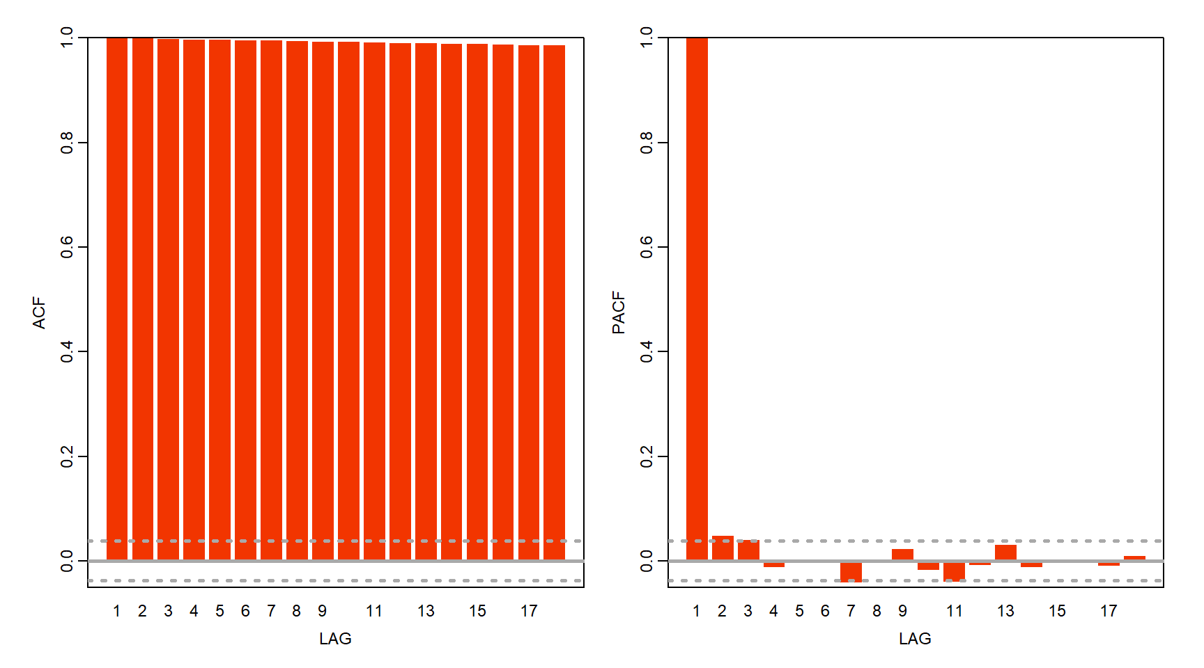
ac(Vo(CORN)) # Volume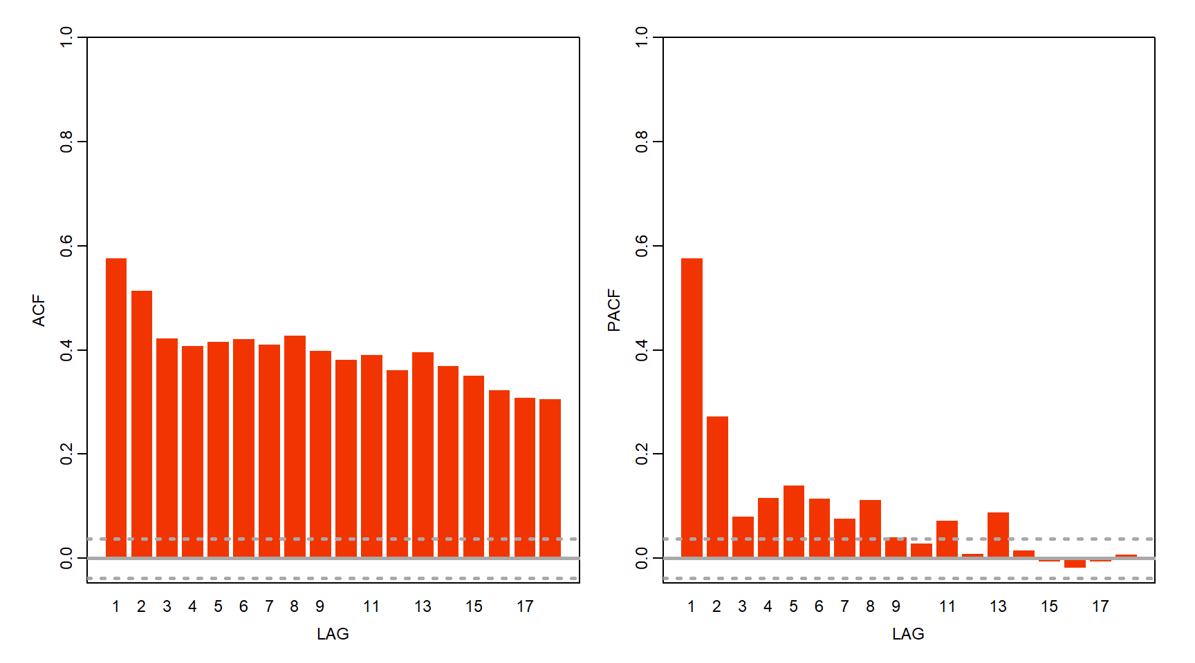
Teste de estacionariedade
Testes de estacionariedade para as séries em nível e em log retornos.
# Phillips-Perron

PP.test(Cl(CORN)) # Fechamento
    Phillips-Perron Unit Root Test

data:  Cl(CORN)
Dickey-Fuller = -3.0462, Truncation lag parameter = 9, p-value = 0.1354
PP.test(Vo(CORN)) # Volume
    Phillips-Perron Unit Root Test

data:  Vo(CORN)
Dickey-Fuller = -32.219, Truncation lag parameter = 9, p-value = 0.01
#PP.test(grupo[,"ret_close"]) # Retornos dos precos
#PP.test(grupo[,"ret_volume"]) # Retornos do volume# Augmented Dickey-Fuller
summary(ur.df(Cl(CORN), type = "trend", selectlags = "AIC")) # Teste ADF para o fechamento
###############################################
# Augmented Dickey-Fuller Test Unit Root Test #
###############################################

Test regression trend


Call:
lm(formula = z.diff ~ z.lag.1 + 1 + tt + z.diff.lag)

Residuals:
    Min      1Q  Median      3Q     Max
-3.8426 -0.1794 -0.0003  0.1612  4.7004

Coefficients:
              Estimate Std. Error t value Pr(>|t|)
(Intercept)  2.200e-01  7.302e-02   3.013  0.00261 **
z.lag.1     -4.964e-03  1.645e-03  -3.017  0.00257 **
tt          -6.628e-05  2.276e-05  -2.912  0.00362 **
z.diff.lag  -4.673e-02  1.894e-02  -2.467  0.01367 *
---
Signif. codes:  0 '***' 0.001 '**' 0.01 '*' 0.05 '.' 0.1 ' ' 1

Residual standard error: 0.4563 on 2774 degrees of freedom
Multiple R-squared:  0.005693,  Adjusted R-squared:  0.004618
F-statistic: 5.294 on 3 and 2774 DF,  p-value: 0.001223


Value of test-statistic is: -3.0174 3.1523 4.6979

Critical values for test statistics:
      1pct  5pct 10pct
tau3 -3.96 -3.41 -3.12
phi2  6.09  4.68  4.03
phi3  8.27  6.25  5.34
summary(ur.df(Vo(CORN), type = "trend", selectlags = "AIC")) # Teste ADF para o volume
###############################################
# Augmented Dickey-Fuller Test Unit Root Test #
###############################################

Test regression trend


Call:
lm(formula = z.diff ~ z.lag.1 + 1 + tt + z.diff.lag)

Residuals:
    Min      1Q  Median      3Q     Max
-988620  -44745  -21243   15092 2533954

Coefficients:
              Estimate Std. Error t value Pr(>|t|)
(Intercept)  1.992e+04  4.768e+03   4.177 3.04e-05 ***
z.lag.1     -3.246e-01  1.725e-02 -18.822  < 2e-16 ***
tt           1.371e+01  2.988e+00   4.588 4.68e-06 ***
z.diff.lag  -2.713e-01  1.827e-02 -14.846  < 2e-16 ***
---
Signif. codes:  0 '***' 0.001 '**' 0.01 '*' 0.05 '.' 0.1 ' ' 1

Residual standard error: 122500 on 2774 degrees of freedom
Multiple R-squared:   0.28, Adjusted R-squared:  0.2792
F-statistic: 359.5 on 3 and 2774 DF,  p-value: < 2.2e-16


Value of test-statistic is: -18.8218 118.0874 177.1304

Critical values for test statistics:
      1pct  5pct 10pct
tau3 -3.96 -3.41 -3.12
phi2  6.09  4.68  4.03
phi3  8.27  6.25  5.34
# KPSS
CORN[,"CORN.Close"] %>% ur.kpss() %>% summary() # Teste para preco de fechamento em nivel
#######################
# KPSS Unit Root Test #
#######################

Test is of type: mu with 9 lags.

Value of test-statistic is: 23.6552

Critical value for a significance level of:
                10pct  5pct 2.5pct  1pct
critical values 0.347 0.463  0.574 0.739
CORN[,"CORN.Volume"] %>% ur.kpss() %>% summary() # Teste para volume em nivel
#######################
# KPSS Unit Root Test #
#######################

Test is of type: mu with 9 lags.

Value of test-statistic is: 2.9658

Critical value for a significance level of:
                10pct  5pct 2.5pct  1pct
critical values 0.347 0.463  0.574 0.739
ret(CORN[,"CORN.Close"],1) %>% ur.kpss() %>% summary() # Teste para retorno dos precos
#######################
# KPSS Unit Root Test #
#######################

Test is of type: mu with 9 lags.

Value of test-statistic is: 0.2531

Critical value for a significance level of:
                10pct  5pct 2.5pct  1pct
critical values 0.347 0.463  0.574 0.739
ret(CORN[,"CORN.Volume"],1) %>% ur.kpss() %>% summary() # Teste para retorno do volume
#######################
# KPSS Unit Root Test #
#######################

Test is of type: mu with 9 lags.

Value of test-statistic is: 0.0194

Critical value for a significance level of:
                10pct  5pct 2.5pct  1pct
critical values 0.347 0.463  0.574 0.739
Seleção das defasagens do modelo
v1 <- cbind(ret(Cl(CORN),1),
            ret(Vo(CORN),1)) # Series em log retornos somente

colnames(v1) <- cbind("ret_cl",
                      "ret_vol")

v1 <- v1[-1,] # Retiro a primeira linha com NA
Transformo para um objeto do tipo ts()
periodicity(v1) # Disponibilidade/range da serie Daily periodicity from 2010-06-10 to 2021-06-23 ret_cl <- ts(ret(Cl(CORN),1), start = c(2010, 6), end = c(2021, 6), frequency = 7)
ret_vo <- ts(ret(Vo(CORN),1), start = c(2010, 6), end = c(2021, 6), frequency = 7)
head(ret_cl)Time Series:
Start = c(2010, 6)
End = c(2011, 4)
Frequency = 7
CORN.Close
[1,] NA
[2,] 0.012250657
[3,] 0.012878305
[4,] 0.012331562
[5,] -0.005376434
[6,] 0.013387119
attr(,"src")
[1] yahoo
attr(,"updated")
[1] 2021-06-24 14:24:34 -03
attr(,"index")
[1] 1276041600 1276128000 1276214400 1276473600 1276560000 1276646400
[7] 1276732800 1276819200 1277078400 1277164800 1277251200 1277337600
[13] 1277424000 1277683200 1277769600 1277856000 1277942400 1278028800
[19] 1278374400 1278460800 1278547200 1278633600 1278892800 1278979200
[25] 1279065600 1279152000 1279238400 1279497600 1279584000 1279670400
[31] 1279756800 1279843200 1280102400 1280188800 1280275200 1280361600
[37] 1280448000 1280707200 1280793600 1280880000 1280966400 1281052800
[43] 1281312000 1281398400 1281484800 1281571200 1281657600 1281916800
[49] 1282003200 1282089600 1282176000 1282262400 1282521600 1282608000
[55] 1282694400 1282780800 1282867200 1283126400 1283212800 1283299200
[61] 1283385600 1283472000 1283817600 1283904000 1283990400 1284076800
[67] 1284336000 1284422400 1284508800 1284595200 1284681600 1284940800
[73] 1285027200 1285113600 1285200000 1285286400 1285545600 1285632000
attr(,"index")attr(,"tzone")
[1] UTC
attr(,"index")attr(,"tclass")
[1] Datetail(ret_cl)Time Series:
Start = c(2021, 1)
End = c(2021, 6)
Frequency = 7
CORN.Close
[1,] -0.005186953
[2,] 0.008832127
[3,] -0.014353644
[4,] 0.036246827
[5,] -0.011636682
[6,] -0.020312900
attr(,"src")
[1] yahoo
attr(,"updated")
[1] 2021-06-24 14:24:34 -03
attr(,"index")
[1] 1276041600 1276128000 1276214400 1276473600 1276560000 1276646400
[7] 1276732800 1276819200 1277078400 1277164800 1277251200 1277337600
[13] 1277424000 1277683200 1277769600 1277856000 1277942400 1278028800
[19] 1278374400 1278460800 1278547200 1278633600 1278892800 1278979200
[25] 1279065600 1279152000 1279238400 1279497600 1279584000 1279670400
[31] 1279756800 1279843200 1280102400 1280188800 1280275200 1280361600
[37] 1280448000 1280707200 1280793600 1280880000 1280966400 1281052800
[43] 1281312000 1281398400 1281484800 1281571200 1281657600 1281916800
[49] 1282003200 1282089600 1282176000 1282262400 1282521600 1282608000
[55] 1282694400 1282780800 1282867200 1283126400 1283212800 1283299200
[61] 1283385600 1283472000 1283817600 1283904000 1283990400 1284076800
[67] 1284336000 1284422400 1284508800 1284595200 1284681600 1284940800
[73] 1285027200 1285113600 1285200000 1285286400 1285545600 1285632000
attr(,"index")attr(,"tzone")
[1] UTC
attr(,"index")attr(,"tclass")
[1] Dateglimpse(ret_cl) Time-Series [1:78, 1] from 2011 to 2022: NA 0.01225 0.01288 0.01233 -0.00538 ...
- attr(*, "src")= chr "yahoo"
- attr(*, "updated")= POSIXct[1:1], format: "2021-06-24 14:24:34"
- attr(*, "index")= num [1:78] 1.28e+09 1.28e+09 1.28e+09 1.28e+09 1.28e+09 ...
..- attr(*, "tzone")= chr "UTC"
..- attr(*, "tclass")= chr "Date"
- attr(*, "dimnames")=List of 2
..$ : NULL
..$ : chr "CORN.Close"Chamo a função pra encontrar a ordem dos lags
lagselect <- VARselect(v1, lag.max = 15, type = "const") # Funcao da ordem das defasagens no modelo VAR
lagselect$selection
AIC(n) HQ(n) SC(n) FPE(n)
11 7 6 11 Estimativa do modelo
Primeiramente estimo ambas as equações separadamente por OLS e usamos coeftest() para obter erros padrão robustos.
VAR_mod <- dynlm(ret_cl ~ ret_vo,
                 start = c(2010, 6),
                 end = c(2021, 6))

coeftest(VAR_mod, vcov. = sandwich)
t test of coefficients:

             Estimate Std. Error t value Pr(>|t|)
(Intercept) 0.0032796  0.0019409  1.6897  0.09524 .
ret_vo      0.0028499  0.0014077  2.0245  0.04648 *
---
Signif. codes:  0 '***' 0.001 '**' 0.01 '*' 0.05 '.' 0.1 ' ' 1
Rodo com a função VAR :
VAR_dados <- window(ts.union(ret_cl, ret_vo), start = c(2010, 6), end = c(2021, 4))

VAR_dados <- VAR_dados[-1,]

glimpse(VAR_dados)
num [1:75, 1:2] 0.01225 0.01288 0.01233 -0.00538 0.01339 ...
- attr(*, "dimnames")=List of 2
..$ : NULL
..$ : chr [1:2] "ret_cl" "ret_vo"VAR_est <- VAR(y = VAR_dados, p = 7) # Lag de 7 dias (memoria de uma semana dos traders)#predict(VAR_est)Análise de resíduos
Serial1 <- serial.test(Model1, lags.pt = 5, type = "PT.asymptotic")
Serial1
[continuar escrevendo…]
Referências