Resumo

Este artigo demonstra um case de aplicação dos modelos de heterocedasticidade condicional para cotações de ativos financeiros (em especial da VALE), com integração via scrapping direto do site do Yahoo!Finance. As cotações apresentam um delay de aproximadamente 1 dia de negociação, e os scripts dos chunks do R estão todos disponíveis para replicações futuras.

A inspiração de usar a News Impact Curve surgiu do meu trabalho de monografia de graduação em Economia na UFPR em 2008, quando o Laboratório de Estatística e Geoinformação (LEG) do departamento de Estatística da Universidade criou um projeto de pesquisa, um wiki, que está disponível até hoje para sua consulta.

Palavras-Chave: ARCH, VALE, News Impact Curve, Econometria

Introdução

Esse relatório capta dinamicamente as cotações de tres ativos

PBR Petrobras
VALE Vale
^BVSP Indice Bovespa

Os dados são originários do Yahoo finance. As séries temporais se iniciam em 01/01/2018 e terminam no último valor de fechamento quase que em real time.

Navegue nele para ver a aplicação de modelos econométricos de volatilidade condicional para os dados da VALE.

Iniciamos observando o caso da maior estatal brasileira, a petrolífera Petrobras:

`PBR` Preço de Fechamento do pregão

`PBR` Volume negociado

A Operação Lava Jato é um conjunto de investigações, algumas controversas, em andamento pela Polícia Federal do Brasil, que cumpriu mais de mil mandados de busca e apreensão, de prisão temporária, de prisão preventiva e de condução coercitiva, visando apurar um esquema de lavagem de dinheiro que movimentou bilhões de reais em propina.

A operação teve início em 17 de março de 2014 e conta com 71 fases operacionais autorizadas, entre outros, pelo então juiz Sérgio Moro, durante as quais prenderam-se e condenaram-se mais de cem pessoas. Investiga crimes de corrupção ativa e passiva, gestão fraudulenta, lavagem de dinheiro, organização criminosa, obstrução da justiça, operação fraudulenta de câmbio e recebimento de vantagem indevida. A Lava Jato foi apontada por críticos como uma das causas da crise político-econômica de 2014 no país. De acordo com investigações e delações premiadas, estavam envolvidos em corrupção membros administrativos da empresa estatal petrolífera Petrobras, políticos dos maiores partidos do Brasil, incluindo presidentes da República, presidentes da Câmara dos Deputados e do Senado Federal e governadores de estados, além de empresários de grandes empresas brasileiras. A Polícia Federal considera-a a maior investigação de corrupção da história do país.

`^BVSP` Preço de Fechamento do pregão

`^BVSP` Volume negociado

O índice bovespa, também chamado de IBOV, é o principal indicador médio de desempenho do mercado de ações no Brasil.

É chamado o “termômetro do mercado de ações”. Se um investidor quer saber como está sua carteira de ações, ele compara com o desempenho do índice bovespa. Se ele está melhor, pior ou com desempenho similar ao do índice.

Formado pela composição de ações das empresas com maior liquidez e maior volume financeiro negociado de todo o volume de negócios da bolsa.

`VALE` Preço de Fechamento do pregão

`VALE` Volume negociado

O rompimento de barragem em Brumadinho em 25 de janeiro de 2019 foi o maior acidente de trabalho no Brasil em perda de vidas humanas e o segundo maior desastre industrial do século. Foi um dos maiores desastres ambientais da mineração do país, depois do rompimento de barragem em Mariana.

Controlada pela Vale S.A., a barragem de rejeitos denominada barragem da Mina Córrego do Feijão, era classificada como de “baixo risco” e “alto potencial de danos” pela empresa. Acumulando os rejeitos de um mina de ferro, ficava no ribeirão Ferro-Carvão, na região de Córrego do Feijão, no município de Brumadinho, estado de Minas Gerais.

Volatilidade Variável no Tempo e Modelos ARCH

O modelo autoregressivo de heterocedasticidade condicional (ARCH) diz respeito a séries temporais com heterocedasticidade variável no tempo, onde a variância é condicional à informação existente em um determinado ponto no tempo.

O modelo ARCH

O modelo ARCH assume que a média condicional do termo de erro em um modelo de série temporal é constante (zero), ao contrário da série não estacionária, mas sua variância condicional não. Esse modelo pode ser descrito como nas Equações 1, 2 e 3.

\[\begin{equation} y_{t}=\phi +e_{t} \label{eq:archdefA14} \end{equation}\]

\[\begin{equation} e_{t} | I_{t-1} \sim N(0,h_{t}) \label{eq:archdefB14} \end{equation}\]

\[\begin{equation} h_{t}=\alpha_{0}+\alpha_{1}e_{t-1}^2, \;\;\;\alpha_{0}>0, \;\; 0\leq \alpha_{1}<1 \label{eq:archdefC14} \end{equation}\]

As Equações 4 e 5 fornecem o modelo de teste e as hipóteses para testar os efeitos ARCH em uma série de tempo, onde os resíduos e \(\hat e_{t}\) vêm da regressão da variável \(y_{t}\) em uma constante, como 1, ou em uma constante mais outros regressores; o teste mostrado na Equação 4 pode incluir vários termos de defasagem, caso em que a hipótese nula (Equação 5) seria que todos eles são conjuntamente insignificantes.

\[\begin{equation} \hat e_{t}^2 = \gamma_{0}+\gamma_{1}\hat e_{t-1}^2+...+\gamma_{q}e_{t-q}^2+\nu_{t} \label{eq:archeffectseqA14} \end{equation}\]

\[\begin{equation} H_{0}:\gamma_{1}=...=\gamma_{q}=0\;\;\;H_{A}:\gamma_{1}\neq 0\;or\;...\gamma_{q}\neq 0 \label{eq:archeffectseqB14} \end{equation}\]

A hipótese nula é que não há efeitos ARCH. A estatística de teste é

\[ (T-q)R^2 \sim \chi ^2_{(1-\alpha,q)} \]

Rodando o modelo ARCH e GARCH para os dados da VALE

ativo2[1:10,] # Gero as primeiras 10 linhas do dataset

           VALE.Open VALE.High VALE.Low VALE.Close VALE.Volume VALE.Adjusted
2018-01-02     12.55     12.80    12.51      12.77    19189400      9.018118
2018-01-03     12.80     12.87    12.68      12.85    20449600      9.074613
2018-01-04     13.03     13.09    12.82      12.83    22033100      9.060488
2018-01-05     12.80     13.09    12.73      13.09    20042800      9.244100
2018-01-08     13.26     13.32    13.18      13.32    17507000      9.406524
2018-01-09     13.40     13.42    13.18      13.24    31204900      9.350030
2018-01-10     13.10     13.21    13.05      13.15    16253500      9.286470
2018-01-11     13.21     13.46    13.20      13.45    15011400      9.498329
2018-01-12     13.51     13.57    13.42      13.53    19012500      9.554827
2018-01-16     13.28     13.31    13.08      13.17    40821800      9.300596

Cl(ativo2) # Gero os dados para aqueles que desejem baixar por aqui

           VALE.Close
2018-01-02      12.77
2018-01-03      12.85
2018-01-04      12.83
2018-01-05      13.09
2018-01-08      13.32
2018-01-09      13.24
2018-01-10      13.15
2018-01-11      13.45
2018-01-12      13.53
2018-01-16      13.17
       ...           
2023-05-26      13.26
2023-05-30      12.76
2023-05-31      12.68
2023-06-01      13.04
2023-06-02      13.68
2023-06-05      13.61
2023-06-06      13.74
2023-06-07      13.94
2023-06-08      14.09
2023-06-09      14.04

Vo(ativo2) # Gero os dados para aqueles que desejem baixar por aqui

           VALE.Volume
2018-01-02    19189400
2018-01-03    20449600
2018-01-04    22033100
2018-01-05    20042800
2018-01-08    17507000
2018-01-09    31204900
2018-01-10    16253500
2018-01-11    15011400
2018-01-12    19012500
2018-01-16    40821800
       ...            
2023-05-26    19326400
2023-05-30    30416300
2023-05-31    45251700
2023-06-01    52730200
2023-06-02    29286200
2023-06-05    18834400
2023-06-06    23116100
2023-06-07    24257200
2023-06-08    15324000
2023-06-09    26761600

# Voce pode usar o seguinte comando para exportar esse dataset 

write.csv(ativo2, file="VALE.csv")


library(xlsx)
write.xlsx(ativo2, file="VALE.xlsx")

#https://www.guru99.com/r-exporting-data.html#1

Após vermos os precos de fechamento e volume, obtenho o log retorno dos precos

dlnVALEclose <- diff(log(Cl(ativo2)), lag=1) #ln(Pt/Pt-1)

dlnVALEclose<-dlnVALEclose[-1,]


presAnnotation <- function(dygraph, x, text) {
  dygraph %>%
    dyAnnotation(x, text, attachAtBottom = TRUE, width = 300, height=20)
}

dygraph(dlnVALEclose, main = "Retornos logarítmicos dos preços de fechamento VALE")%>%
   dyAnnotation("2019-01-25", text = "A", tooltip = "Rompimento da barragem em Brumadinho")%>%
presAnnotation("2019-01-25", text = "Rompimento da barragem em Brumadinho")%>%
  dyShading(from = "2019-01-25", to = "2019-02-26")%>%
  dyAnnotation("2020-03-02", text = "A", tooltip = "Corona Day")%>%
presAnnotation("2020-03-02", text = "Corona Day")%>%   
  dyShading(from = "2020-03-02", to = "2020-04-27")

  #Grafico dos retornos

Agora observo o padrão da distribuição dos log retornos:

hist(dlnVALEclose, main="", breaks=20, freq=FALSE, col="grey")
lines(density(dlnVALEclose, adjust=2, col="blue"))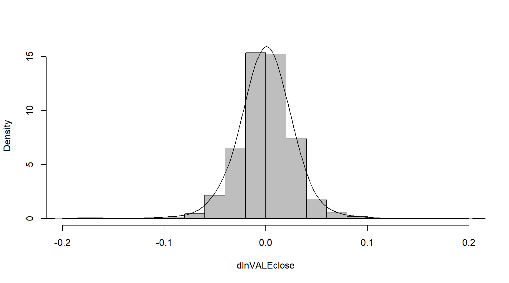

Vamos iniciar carregando os pacotes necessários do R:

#rm(list=ls()) #Removes all items in Environment!
library(FinTS) #for function `ArchTest()`
library(rugarch) #for GARCH models
library(tseries) # for `adf.test()`
library(dynlm) #for function `dynlm()`
library(vars) # for function `VAR()`
library(nlWaldTest) # for the `nlWaldtest()` function
library(lmtest) #for `coeftest()` and `bptest()`.
library(broom) #for `glance(`) and `tidy()`
#library(PoEdata) #for PoE4 datasets
library(car) #for `hccm()` robust standard errors
library(sandwich)
library(knitr) #for `kable()`
library(forecast)

Vamos primeiro realizar, passo a passo, o teste ARCH na variável VALE.Close. Iremos transformar os dados numa série temporal para leitura do R:

library(dynlm)

rTS <- ts(dlnVALEclose) # A funcao ts eh o mesmo que timeseries

plot.ts(ativo2$VALE.Close) # Serie temporal de valor de fechamento da VALE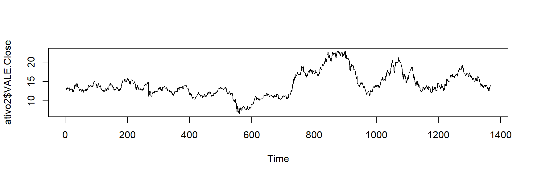

plot.ts(rTS) # Serie de retornos logaritmizados da VALE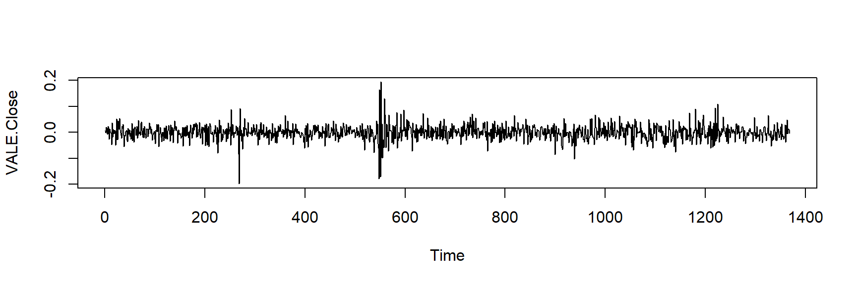

Então obtemos os valores de estimativas dos parâmetros da regressão:

VALE.media <- dynlm(rTS~1)


	Dependent variable:

	rTS

Constant	0.0001
	(0.001)


Observations	1,368
R²	0.000
Adjusted R²	0.000

Note:	p<0.1; p<0.05; p<0.01

ehatsq <- ts(resid(VALE.media)^2) # Obtenho os valores da serie de residuos do modelo ARCH elevado ao quadrado

VALE.ARCH <- dynlm(ehatsq~L(ehatsq)) # Agora estimo o modelo dinamico usando a serie de residuos

summary(VALE.ARCH) # Printa os resultados


Time series regression with "ts" data:
Start = 2, End = 1368

Call:
dynlm(formula = ehatsq ~ L(ehatsq))

Residuals:
      Min        1Q    Median        3Q       Max 
-0.016531 -0.000548 -0.000380  0.000108  0.035992 

Coefficients:
             Estimate Std. Error t value Pr(>|t|)    
(Intercept) 4.591e-04  6.108e-05   7.517 1.01e-13 ***
L(ehatsq)   4.227e-01  2.453e-02  17.234  < 2e-16 ***
---
Signif. codes:  0 '***' 0.001 '**' 0.01 '*' 0.05 '.' 0.1 ' ' 1

Residual standard error: 0.00214 on 1365 degrees of freedom
Multiple R-squared:  0.1787,    Adjusted R-squared:  0.1781 
F-statistic:   297 on 1 and 1365 DF,  p-value: < 2.2e-16


	Dependent variable:

	ehatsq

Constant	0.0005^***
	(0.0001)

L(ehatsq)	0.423^***
	(0.025)


Observations	1,367
R²	0.179
Adjusted R²	0.178

Note:	p<0.1; p<0.05; p<0.01

library(broom)

T <- nobs(VALE.media)

q <- length(coef(VALE.ARCH))-1

Rsq <- glance(VALE.ARCH)[[1]]

LM <- (T-q)*Rsq

alpha <- 0.05

quiquadr <- qchisq(1-alpha, q)

O valor da estatística LM é de 244.3 que deve ser comparado ao valor crítico do qui-quadrado com \(\alpha = 0,05\) e \(q=\) 1 grau de liberdade; este valor é \(\chi^{2}_{(0,95,\,\, 1)}\) = 3.84; isso indica que a hipótese nula é rejeitada, concluindo que a série tem efeitos ARCH.

A mesma conclusão pode ser alcançada se, em vez do procedimento passo a passo, usarmos um dos recursos de teste ARCH do R, a função ArchTest() no pacote FinTS.

library(FinTS)
VALEArchTest <- ArchTest(dlnVALEclose, lags=1, demean=TRUE)
VALEArchTest


    ARCH LM-test; Null hypothesis: no ARCH effects

data:  dlnVALEclose
Chi-squared = 244.3, df = 1, p-value < 2.2e-16

A função garch() no pacote tseries torna-se um modelo ARCH quando usada com o order = argumento igual a c(0,1). Essa função pode ser usada para estimar e plotar a variância \(h_{t}\) definida na Equação 3, conforme mostrado no código a seguir e na Figura abaixo.

library(tseries)

rTS<-rTS%>%
  na.omit() # Retiro os NAs da serie

VALE.arch <- garch(rTS,c(0,1))


 ***** ESTIMATION WITH ANALYTICAL GRADIENT ***** 

     I     INITIAL X(I)        D(I)

     1     7.555777e-04     1.000e+00
     2     5.000000e-02     1.000e+00

    IT   NF      F         RELDF    PRELDF    RELDX   STPPAR   D*STEP   NPRELDF
     0    1 -4.247e+03
     1    6 -4.252e+03  9.97e-04  2.18e-03  1.0e-03  9.3e+08  1.0e-04  1.01e+06
     2    7 -4.252e+03  3.77e-05  4.69e-05  9.9e-04  2.0e+00  1.0e-04  3.39e+01
     3   13 -4.271e+03  4.53e-03  7.62e-03  3.8e-01  2.0e+00  6.1e-02  3.38e+01
     4   15 -4.273e+03  4.84e-04  1.16e-03  7.8e-02  1.1e+00  1.9e-02  1.85e-03
     5   17 -4.279e+03  1.25e-03  8.55e-04  1.2e-01  0.0e+00  3.7e-02  8.55e-04
     6   18 -4.281e+03  4.69e-04  4.06e-04  1.0e-01  1.8e-01  3.7e-02  4.15e-04
     7   19 -4.281e+03  1.54e-04  1.17e-04  6.3e-02  0.0e+00  2.8e-02  1.17e-04
     8   20 -4.281e+03  2.52e-05  2.17e-05  2.9e-02  0.0e+00  1.4e-02  2.17e-05
     9   21 -4.281e+03  9.45e-07  8.79e-07  6.5e-03  0.0e+00  3.2e-03  8.79e-07
    10   22 -4.281e+03  6.37e-09  6.26e-09  5.8e-04  0.0e+00  2.9e-04  6.26e-09
    11   23 -4.281e+03  2.56e-12  2.53e-12  1.1e-05  0.0e+00  5.4e-06  2.53e-12

 ***** RELATIVE FUNCTION CONVERGENCE *****

 FUNCTION    -4.281430e+03   RELDX        1.083e-05
 FUNC. EVALS      23         GRAD. EVALS      12
 PRELDF       2.526e-12      NPRELDF      2.526e-12

     I      FINAL X(I)        D(I)          G(I)

     1    5.627445e-04     1.000e+00     1.828e-01
     2    2.475817e-01     1.000e+00     4.131e-05

sbydarch <- summary(VALE.arch)
sbydarch


Call:
garch(x = rTS, order = c(0, 1))

Model:
GARCH(0,1)

Residuals:
     Min       1Q   Median       3Q      Max 
-4.68465 -0.59037  0.02321  0.59399  4.37563 

Coefficient(s):
    Estimate  Std. Error  t value Pr(>|t|)    
a0 5.627e-04   2.198e-05     25.6   <2e-16 ***
a1 2.476e-01   2.293e-02     10.8   <2e-16 ***
---
Signif. codes:  0 '***' 0.001 '**' 0.01 '*' 0.05 '.' 0.1 ' ' 1

Diagnostic Tests:
    Jarque Bera Test

data:  Residuals
X-squared = 134.77, df = 2, p-value < 2.2e-16


    Box-Ljung test

data:  Squared.Residuals
X-squared = 0.024545, df = 1, p-value = 0.8755

hhat <- ts(2*VALE.arch$fitted.values[-1,1]^2)

plot.ts(hhat)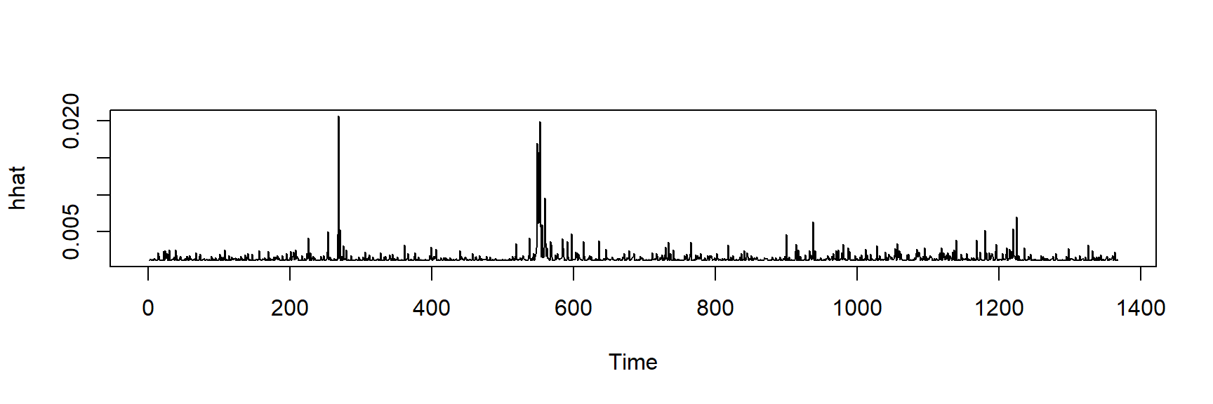

O modelo GARCH

library(rugarch)
garchSpec <- ugarchspec(
           variance.model=list(model="sGARCH",
                               garchOrder=c(1,1)),
           mean.model=list(armaOrder=c(0,0)), 
           distribution.model="std")
garchFit <- ugarchfit(spec=garchSpec, data=rTS)
coef(garchFit)

          mu        omega       alpha1        beta1        shape 
5.098919e-04 8.181086e-05 7.732878e-02 8.075895e-01 6.563801e+00

rhat <- garchFit@fit$fitted.values
plot.ts(rhat)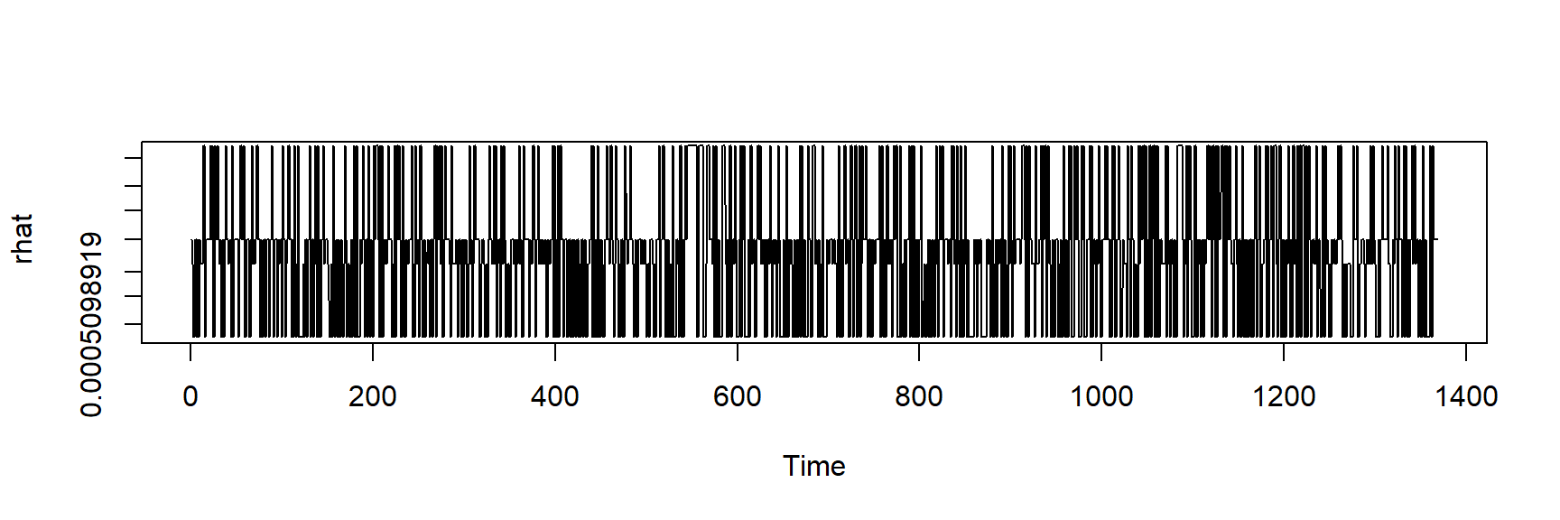

hhat <- ts(garchFit@fit$sigma^2)
plot.ts(hhat)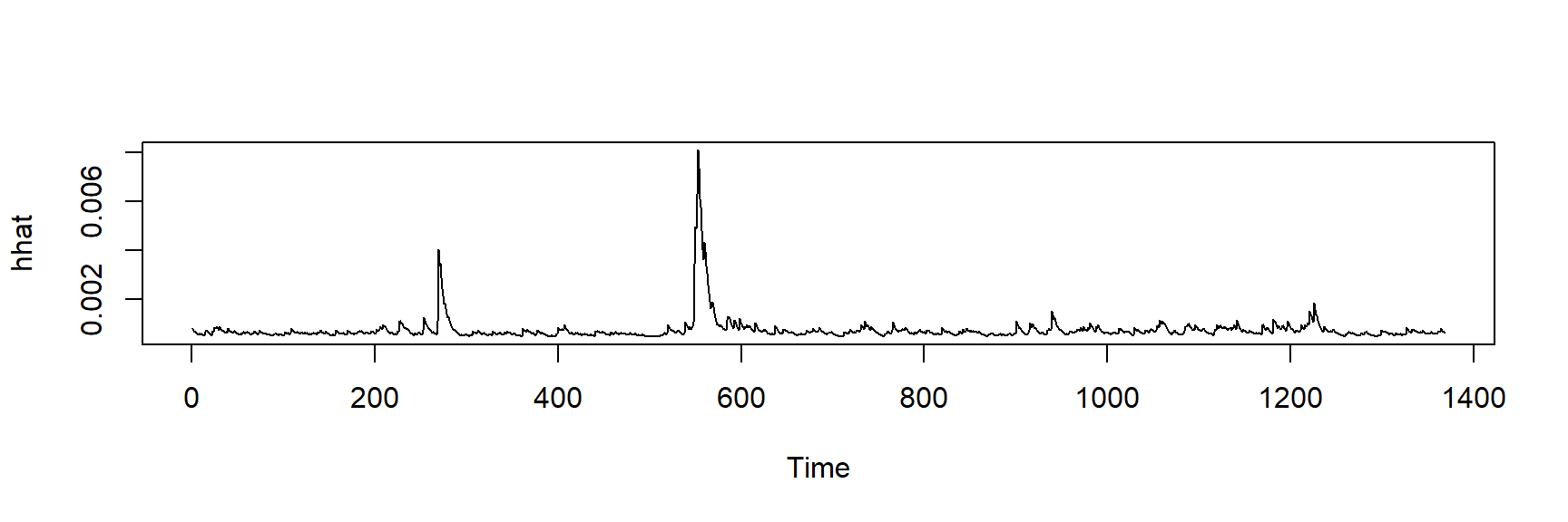

# tGARCH 
garchMod <- ugarchspec(variance.model=list(model="fGARCH",
                               garchOrder=c(1,1),
                               submodel="TGARCH"),
           mean.model=list(armaOrder=c(0,0)), 
           distribution.model="std")
garchFit <- ugarchfit(spec=garchMod, data=rTS)
coef(garchFit)

          mu        omega       alpha1        beta1        eta11        shape 
0.0001448778 0.0024951666 0.0829903566 0.8426163519 0.6037352495 6.7955576554

rhat <- garchFit@fit$fitted.values
plot.ts(rhat)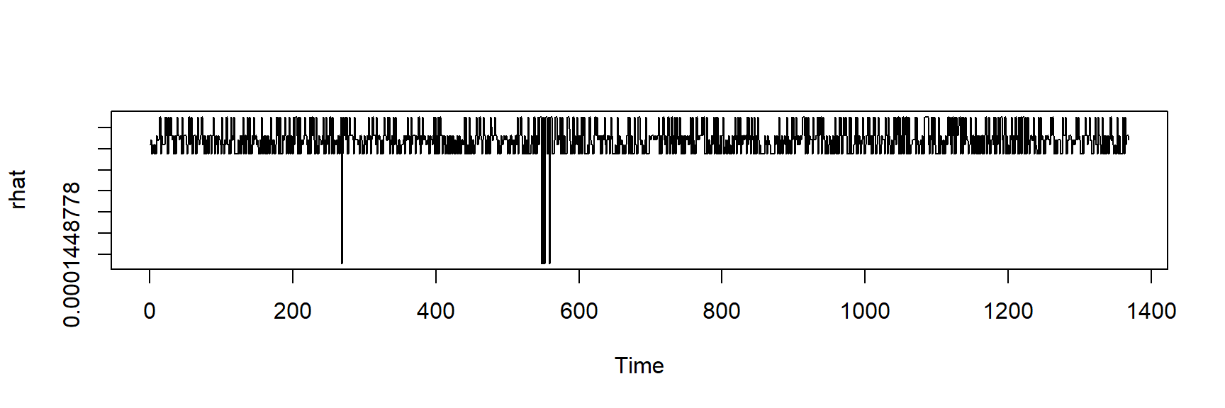

hhat <- ts(garchFit@fit$sigma^2)
plot.ts(hhat)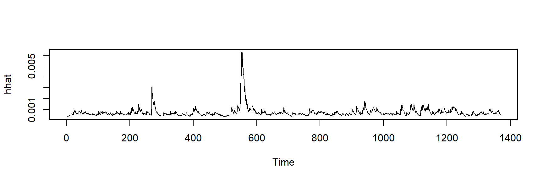

# GARCH-in-mean
garchMod <- ugarchspec(
          variance.model=list(model="fGARCH",
                               garchOrder=c(1,1),
                               submodel="APARCH"),
           mean.model=list(armaOrder=c(0,0),
                          include.mean=TRUE,
                          archm=TRUE,
                          archpow=2
                          ), 
           distribution.model="std"
                           )
garchFit <- ugarchfit(spec=garchMod, data=rTS)
coef(garchFit)

          mu        archm        omega       alpha1        beta1        eta11 
-0.001572400  2.693463496  0.001299905  0.083006027  0.814291951  0.578064680 
      lambda        shape 
 1.237831744  6.936388133

rhat <- garchFit@fit$fitted.values
plot.ts(rhat)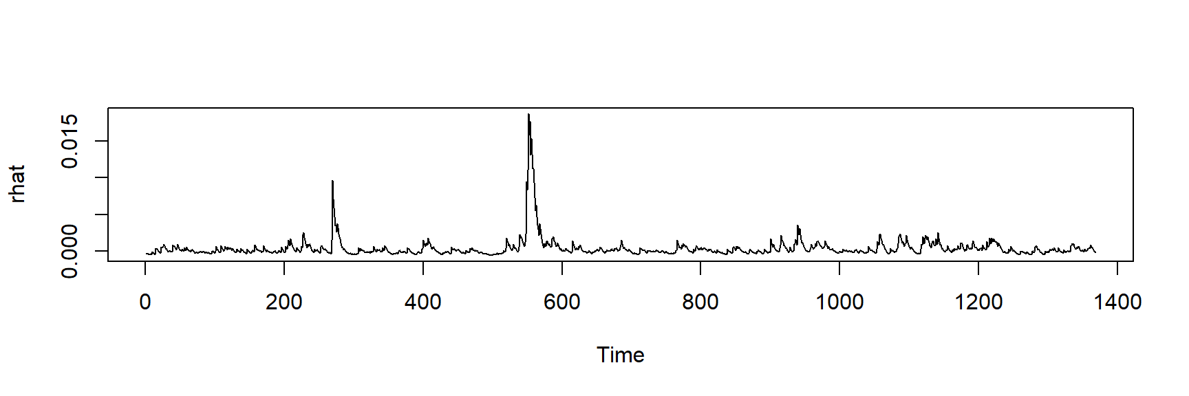

hhat <- ts(garchFit@fit$sigma^2)
plot.ts(hhat)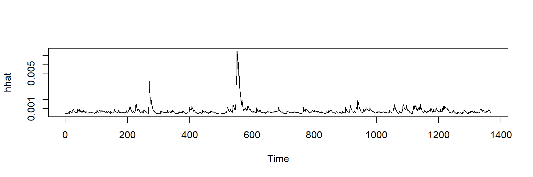

As Figuras anteriores mostram algumas versões do modelo GARCH. As previsões podem ser obtidas usando a função ugarchboot() do pacote ugarch.

Outro script para a News Impact Curve

library(PerformanceAnalytics)
library(quantmod)
library(rugarch)
library(car)
library(FinTS)

options(digits=4)

VALEfechamento<-ativo2$VALE.Close

# Calcula o log retorno dos precos de fechamento da VALE
VALE.ret = CalculateReturns(VALEfechamento, method="log")

VALE.ret[1:10,] # printa as primeiras dez linhas

           VALE.Close
2018-01-02         NA
2018-01-03   0.006245
2018-01-04  -0.001558
2018-01-05   0.020062
2018-01-08   0.017418
2018-01-09  -0.006024
2018-01-10  -0.006821
2018-01-11   0.022557
2018-01-12   0.005930
2018-01-16  -0.026968

VALE.ret=VALE.ret[-1,] # Removo o primeiro NA

VALE.ret[1:10,] # printa as primeiras dez linhas

           VALE.Close
2018-01-03   0.006245
2018-01-04  -0.001558
2018-01-05   0.020062
2018-01-08   0.017418
2018-01-09  -0.006024
2018-01-10  -0.006821
2018-01-11   0.022557
2018-01-12   0.005930
2018-01-16  -0.026968
2018-01-17   0.013575

GARCH Assimétrico

Agora vamos definir o GARCH assimétrico

garch11.spec = ugarchspec(variance.model = list(garchOrder=c(1,1)), 
                          mean.model = list(armaOrder=c(0,0)))
VALE.garch11.fit = ugarchfit(spec=garch11.spec, data=VALE.ret,
                             solver.control=list(trace = 1))


Iter: 1 fn: -3045.0634   Pars:  0.0005617 0.0001112 0.1226330 0.7247662
Iter: 2 fn: -3045.0634   Pars:  0.0005616 0.0001112 0.1226429 0.7247721
solnp--> Completed in 2 iterations

VALE.garch11.fit


*---------------------------------*
*          GARCH Model Fit        *
*---------------------------------*

Conditional Variance Dynamics   
-----------------------------------
GARCH Model : sGARCH(1,1)
Mean Model  : ARFIMA(0,0,0)
Distribution    : norm 

Optimal Parameters
------------------------------------
        Estimate  Std. Error  t value Pr(>|t|)
mu      0.000562    0.000676  0.83051 0.406253
omega   0.000111    0.000034  3.27136 0.001070
alpha1  0.122643    0.024780  4.94933 0.000001
beta1   0.724772    0.063199 11.46801 0.000000

Robust Standard Errors:
        Estimate  Std. Error  t value Pr(>|t|)
mu      0.000562    0.000667  0.84239 0.399568
omega   0.000111    0.000060  1.84512 0.065019
alpha1  0.122643    0.059972  2.04499 0.040856
beta1   0.724772    0.124365  5.82780 0.000000

LogLikelihood : 3045 

Information Criteria
------------------------------------
                    
Akaike       -4.4460
Bayes        -4.4307
Shibata      -4.4460
Hannan-Quinn -4.4403

Weighted Ljung-Box Test on Standardized Residuals
------------------------------------
                        statistic p-value
Lag[1]                    0.01975  0.8882
Lag[2*(p+q)+(p+q)-1][2]   0.23233  0.8346
Lag[4*(p+q)+(p+q)-1][5]   1.50811  0.7379
d.o.f=0
H0 : No serial correlation

Weighted Ljung-Box Test on Standardized Squared Residuals
------------------------------------
                        statistic  p-value
Lag[1]                      6.808 0.009077
Lag[2*(p+q)+(p+q)-1][5]     7.745 0.034073
Lag[4*(p+q)+(p+q)-1][9]     9.341 0.069102
d.o.f=2

Weighted ARCH LM Tests
------------------------------------
            Statistic Shape Scale P-Value
ARCH Lag[3]     0.090 0.500 2.000  0.7642
ARCH Lag[5]     1.151 1.440 1.667  0.6888
ARCH Lag[7]     1.996 2.315 1.543  0.7181

Nyblom stability test
------------------------------------
Joint Statistic:  0.6963
Individual Statistics:              
mu     0.05934
omega  0.17910
alpha1 0.07439
beta1  0.20613

Asymptotic Critical Values (10% 5% 1%)
Joint Statistic:         1.07 1.24 1.6
Individual Statistic:    0.35 0.47 0.75

Sign Bias Test
------------------------------------
                   t-value     prob sig
Sign Bias           1.1389 0.254925    
Negative Sign Bias  3.1327 0.001769 ***
Positive Sign Bias  0.8256 0.409155    
Joint Effect       12.0285 0.007286 ***


Adjusted Pearson Goodness-of-Fit Test:
------------------------------------
  group statistic p-value(g-1)
1    20     38.67     0.004877
2    30     43.18     0.043775
3    40     57.32     0.029368
4    50     72.64     0.015750


Elapsed time : 0.1835

plot(residuals(VALE.garch11.fit))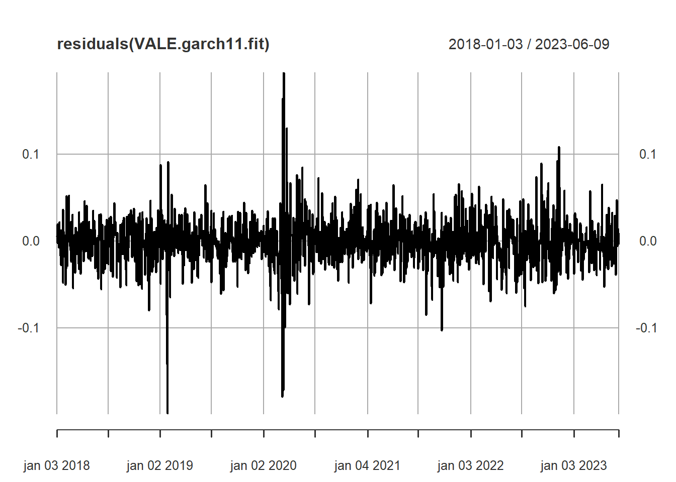

Rodaremos o teste de Engle & NG. para o viés de sinal:

O teste de viés de sinal considera a variável \(S_{t-1}^{-}\), uma variável fictícia que assume o valor um quando \(\epsilon_{t-1}\) é negativo e zero, caso contrário. Este teste examina o impacto de choques de retorno positivo e negativo sobre a volatilidade não prevista pelo modelo em consideração. O teste de viés de tamanho negativo utiliza a variável \(S_{t-1}^{-}\) \(\epsilon_{t-1}\). Ele se concentra nos diferentes efeitos que grandes e pequenos choques de retorno negativo têm sobre a volatilidade, o que não é previsto pelo modelo de volatilidade. O teste de viés de tamanho positivo utiliza a variável \(S_{t-1}^{+}\) \(\epsilon_{t-1}\) onde \(S_{t-1}^{+}\) é definido como 1 menos \(S_{t-1}\). Ele se concentra nos diferentes impactos que grandes e pequenos choques de retorno positivo podem ter sobre a volatilidade, que não são explicados pelo modelo de volatilidade.

signbias(VALE.garch11.fit)

                   t-value     prob sig
Sign Bias           1.1389 0.254925    
Negative Sign Bias  3.1327 0.001769 ***
Positive Sign Bias  0.8256 0.409155    
Joint Effect       12.0285 0.007286 ***

Como apontado acima, o efeito de viés de negativo foi o que apresentou significância.

Modelo EGARCH de Nelson

egarch11.spec = ugarchspec(variance.model=list(model="eGARCH",
                                               garchOrder=c(1,1)),
                           mean.model=list(armaOrder=c(0,0)))
VALE.egarch11.fit = ugarchfit(egarch11.spec, VALE.ret)
VALE.egarch11.fit


*---------------------------------*
*          GARCH Model Fit        *
*---------------------------------*

Conditional Variance Dynamics   
-----------------------------------
GARCH Model : eGARCH(1,1)
Mean Model  : ARFIMA(0,0,0)
Distribution    : norm 

Optimal Parameters
------------------------------------
        Estimate  Std. Error  t value Pr(>|t|)
mu     -0.000209    0.000671 -0.31211 0.754954
omega  -0.944470    0.262859 -3.59307 0.000327
alpha1 -0.132769    0.027603 -4.80997 0.000002
beta1   0.869359    0.036082 24.09385 0.000000
gamma1  0.213962    0.035379  6.04777 0.000000

Robust Standard Errors:
        Estimate  Std. Error  t value Pr(>|t|)
mu     -0.000209    0.000705  -0.2969 0.766544
omega  -0.944470    0.573335  -1.6473 0.099491
alpha1 -0.132769    0.059557  -2.2293 0.025796
beta1   0.869359    0.079300  10.9629 0.000000
gamma1  0.213962    0.076979   2.7795 0.005445

LogLikelihood : 3054 

Information Criteria
------------------------------------
                    
Akaike       -4.4573
Bayes        -4.4382
Shibata      -4.4573
Hannan-Quinn -4.4501

Weighted Ljung-Box Test on Standardized Residuals
------------------------------------
                        statistic p-value
Lag[1]                  3.039e-06  0.9986
Lag[2*(p+q)+(p+q)-1][2] 1.742e-01  0.8703
Lag[4*(p+q)+(p+q)-1][5] 1.226e+00  0.8068
d.o.f=0
H0 : No serial correlation

Weighted Ljung-Box Test on Standardized Squared Residuals
------------------------------------
                        statistic p-value
Lag[1]                      6.503 0.01077
Lag[2*(p+q)+(p+q)-1][5]     6.939 0.05367
Lag[4*(p+q)+(p+q)-1][9]     8.567 0.09955
d.o.f=2

Weighted ARCH LM Tests
------------------------------------
            Statistic Shape Scale P-Value
ARCH Lag[3]   0.09855 0.500 2.000  0.7536
ARCH Lag[5]   0.49815 1.440 1.667  0.8842
ARCH Lag[7]   1.95431 2.315 1.543  0.7270

Nyblom stability test
------------------------------------
Joint Statistic:  0.8103
Individual Statistics:             
mu     0.1289
omega  0.1249
alpha1 0.1322
beta1  0.1188
gamma1 0.2905

Asymptotic Critical Values (10% 5% 1%)
Joint Statistic:         1.28 1.47 1.88
Individual Statistic:    0.35 0.47 0.75

Sign Bias Test
------------------------------------
                   t-value    prob sig
Sign Bias          1.19739 0.23136    
Negative Sign Bias 2.22994 0.02591  **
Positive Sign Bias 0.05336 0.95745    
Joint Effect       4.99000 0.17253    


Adjusted Pearson Goodness-of-Fit Test:
------------------------------------
  group statistic p-value(g-1)
1    20     33.23      0.02262
2    30     44.98      0.02954
3    40     50.36      0.10506
4    50     69.35      0.02935


Elapsed time : 0.1737

plot(residuals(VALE.egarch11.fit))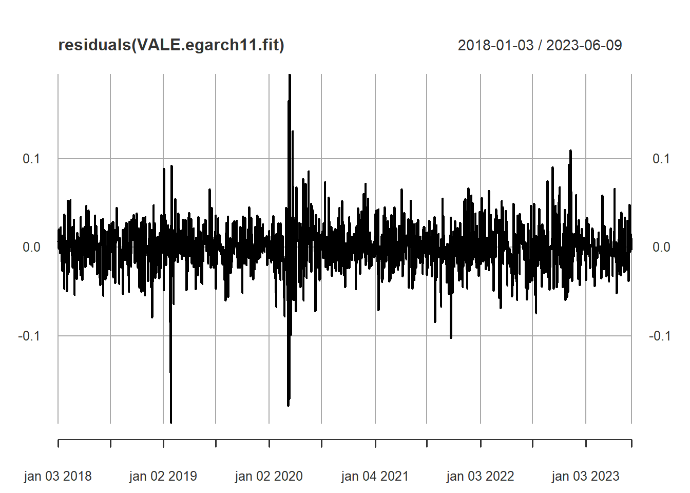

Modelo GJR GARCH

gjrgarch11.spec = ugarchspec(variance.model=list(model="gjrGARCH",
                                                 garchOrder=c(1,1)),
                             mean.model=list(armaOrder=c(0,0)))
VALE.gjrgarch11.fit = ugarchfit(gjrgarch11.spec, VALE.ret)
VALE.gjrgarch11.fit


*---------------------------------*
*          GARCH Model Fit        *
*---------------------------------*

Conditional Variance Dynamics   
-----------------------------------
GARCH Model : gjrGARCH(1,1)
Mean Model  : ARFIMA(0,0,0)
Distribution    : norm 

Optimal Parameters
------------------------------------
        Estimate  Std. Error   t value Pr(>|t|)
mu      0.000047    0.000677  0.068915 0.945057
omega   0.000128    0.000032  4.002958 0.000063
alpha1  0.013622    0.021287  0.639913 0.522229
beta1   0.711888    0.056802 12.532797 0.000000
gamma1  0.192620    0.046233  4.166272 0.000031

Robust Standard Errors:
        Estimate  Std. Error  t value Pr(>|t|)
mu      0.000047    0.000702  0.06647 0.947004
omega   0.000128    0.000056  2.29011 0.022015
alpha1  0.013622    0.021603  0.63055 0.528333
beta1   0.711888    0.102368  6.95423 0.000000
gamma1  0.192620    0.094309  2.04243 0.041109

LogLikelihood : 3057 

Information Criteria
------------------------------------
                    
Akaike       -4.4618
Bayes        -4.4427
Shibata      -4.4618
Hannan-Quinn -4.4547

Weighted Ljung-Box Test on Standardized Residuals
------------------------------------
                        statistic p-value
Lag[1]                   0.007495  0.9310
Lag[2*(p+q)+(p+q)-1][2]  0.098210  0.9209
Lag[4*(p+q)+(p+q)-1][5]  1.211921  0.8101
d.o.f=0
H0 : No serial correlation

Weighted Ljung-Box Test on Standardized Squared Residuals
------------------------------------
                        statistic p-value
Lag[1]                      3.171 0.07496
Lag[2*(p+q)+(p+q)-1][5]     4.090 0.24311
Lag[4*(p+q)+(p+q)-1][9]     6.367 0.25817
d.o.f=2

Weighted ARCH LM Tests
------------------------------------
            Statistic Shape Scale P-Value
ARCH Lag[3]    0.2943 0.500 2.000  0.5875
ARCH Lag[5]    1.1262 1.440 1.667  0.6959
ARCH Lag[7]    3.0940 2.315 1.543  0.4960

Nyblom stability test
------------------------------------
Joint Statistic:  0.9498
Individual Statistics:             
mu     0.1273
omega  0.2589
alpha1 0.1830
beta1  0.3513
gamma1 0.1092

Asymptotic Critical Values (10% 5% 1%)
Joint Statistic:         1.28 1.47 1.88
Individual Statistic:    0.35 0.47 0.75

Sign Bias Test
------------------------------------
                   t-value   prob sig
Sign Bias           0.6108 0.5414    
Negative Sign Bias  1.5094 0.1314    
Positive Sign Bias  0.2721 0.7856    
Joint Effect        2.3523 0.5026    


Adjusted Pearson Goodness-of-Fit Test:
------------------------------------
  group statistic p-value(g-1)
1    20     33.81      0.01933
2    30     39.41      0.09401
3    40     49.37      0.12351
4    50     64.75      0.06522


Elapsed time : 0.3573

plot(residuals(VALE.gjrgarch11.fit))

Modelo APARCH

aparch11.1.spec = ugarchspec(variance.model=list(model="apARCH",
                                                 garchOrder=c(1,1)),
                             mean.model=list(armaOrder=c(0,0)),
                             fixed.pars=list(delta=1))

VALE.aparch11.1.fit = ugarchfit(aparch11.1.spec, VALE.ret)
VALE.aparch11.1.fit


*---------------------------------*
*          GARCH Model Fit        *
*---------------------------------*

Conditional Variance Dynamics   
-----------------------------------
GARCH Model : apARCH(1,1)
Mean Model  : ARFIMA(0,0,0)
Distribution    : norm 

Optimal Parameters
------------------------------------
        Estimate  Std. Error  t value Pr(>|t|)
mu     -0.000214    0.000673 -0.31766 0.750739
omega   0.004021    0.001095  3.67160 0.000241
alpha1  0.116203    0.020798  5.58731 0.000000
beta1   0.760789    0.051128 14.87997 0.000000
gamma1  0.653656    0.150914  4.33131 0.000015
delta   1.000000          NA       NA       NA

Robust Standard Errors:
        Estimate  Std. Error  t value Pr(>|t|)
mu     -0.000214    0.000703 -0.30417 0.761000
omega   0.004021    0.002296  1.75105 0.079937
alpha1  0.116203    0.042770  2.71689 0.006590
beta1   0.760789    0.112343  6.77204 0.000000
gamma1  0.653656    0.166548  3.92472 0.000087
delta   1.000000          NA       NA       NA

LogLikelihood : 3054 

Information Criteria
------------------------------------
                    
Akaike       -4.4573
Bayes        -4.4382
Shibata      -4.4573
Hannan-Quinn -4.4501

Weighted Ljung-Box Test on Standardized Residuals
------------------------------------
                        statistic p-value
Lag[1]                   0.001546  0.9686
Lag[2*(p+q)+(p+q)-1][2]  0.251705  0.8232
Lag[4*(p+q)+(p+q)-1][5]  1.405315  0.7632
d.o.f=0
H0 : No serial correlation

Weighted Ljung-Box Test on Standardized Squared Residuals
------------------------------------
                        statistic  p-value
Lag[1]                      9.593 0.001953
Lag[2*(p+q)+(p+q)-1][5]     9.929 0.009601
Lag[4*(p+q)+(p+q)-1][9]    11.523 0.023244
d.o.f=2

Weighted ARCH LM Tests
------------------------------------
            Statistic Shape Scale P-Value
ARCH Lag[3]   0.06548 0.500 2.000  0.7980
ARCH Lag[5]   0.59218 1.440 1.667  0.8561
ARCH Lag[7]   1.97026 2.315 1.543  0.7236

Nyblom stability test
------------------------------------
Joint Statistic:  0.7544
Individual Statistics:              
mu     0.13466
omega  0.08956
alpha1 0.09893
beta1  0.10852
gamma1 0.12171

Asymptotic Critical Values (10% 5% 1%)
Joint Statistic:         1.28 1.47 1.88
Individual Statistic:    0.35 0.47 0.75

Sign Bias Test
------------------------------------
                    t-value    prob sig
Sign Bias          1.461350 0.14415    
Negative Sign Bias 2.570240 0.01027  **
Positive Sign Bias 0.002776 0.99779    
Joint Effect       6.651720 0.08387   *


Adjusted Pearson Goodness-of-Fit Test:
------------------------------------
  group statistic p-value(g-1)
1    20     35.42     0.012422
2    30     43.97     0.036913
3    40     50.54     0.102050
4    50     75.06     0.009726


Elapsed time : 0.4172

plot(residuals(VALE.aparch11.1.fit))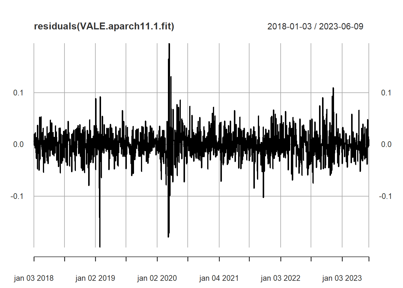

Comparando as News Impact Curves

nic.garch11 = newsimpact(VALE.garch11.fit)
nic.egarch11 = newsimpact(VALE.egarch11.fit)
nic.gjrgarch11 = newsimpact(VALE.gjrgarch11.fit)
nic.aparch11.1 = newsimpact(VALE.aparch11.1.fit)

Via critério de informação, comparamos:

model.list = list(garch11 = VALE.garch11.fit,
                  egarch11 = VALE.egarch11.fit,
                  gjrgarch11 = VALE.gjrgarch11.fit,
                  aparch11.1 = VALE.aparch11.1.fit)
info.mat = sapply(model.list, infocriteria)
rownames(info.mat) = rownames(infocriteria(VALE.garch11.fit))
info.mat

             garch11 egarch11 gjrgarch11 aparch11.1
Akaike        -4.446   -4.457     -4.462     -4.457
Bayes         -4.431   -4.438     -4.443     -4.438
Shibata       -4.446   -4.457     -4.462     -4.457
Hannan-Quinn  -4.440   -4.450     -4.455     -4.450

Mostra a News Impact Curve estimada GARCH(1,1) e EGARCH(1,1)

par(mfrow=c(2,2))
plot(nic.garch11$zx, type="l", lwd=2, col="blue", main="GARCH(1,1)", 
     nic.garch11$zy, ylab=nic.garch11$yexpr, xlab=nic.garch11$xexpr)
plot(nic.egarch11$zx, type="l", lwd=2, col="blue", main="EGARCH(1,1)", 
     nic.egarch11$zy, ylab=nic.egarch11$yexpr, xlab=nic.egarch11$xexpr)
plot(nic.gjrgarch11$zx, type="l", lwd=2, col="blue", main="TGARCH(1,1)", 
     nic.gjrgarch11$zy, ylab=nic.gjrgarch11$yexpr, xlab=nic.gjrgarch11$xexpr)
plot(nic.aparch11.1$zx, type="l", lwd=2, col="blue", main="APARCH(1,1,1)", 
     nic.aparch11.1$zy, ylab=nic.aparch11.1$yexpr, xlab=nic.aparch11.1$xexpr)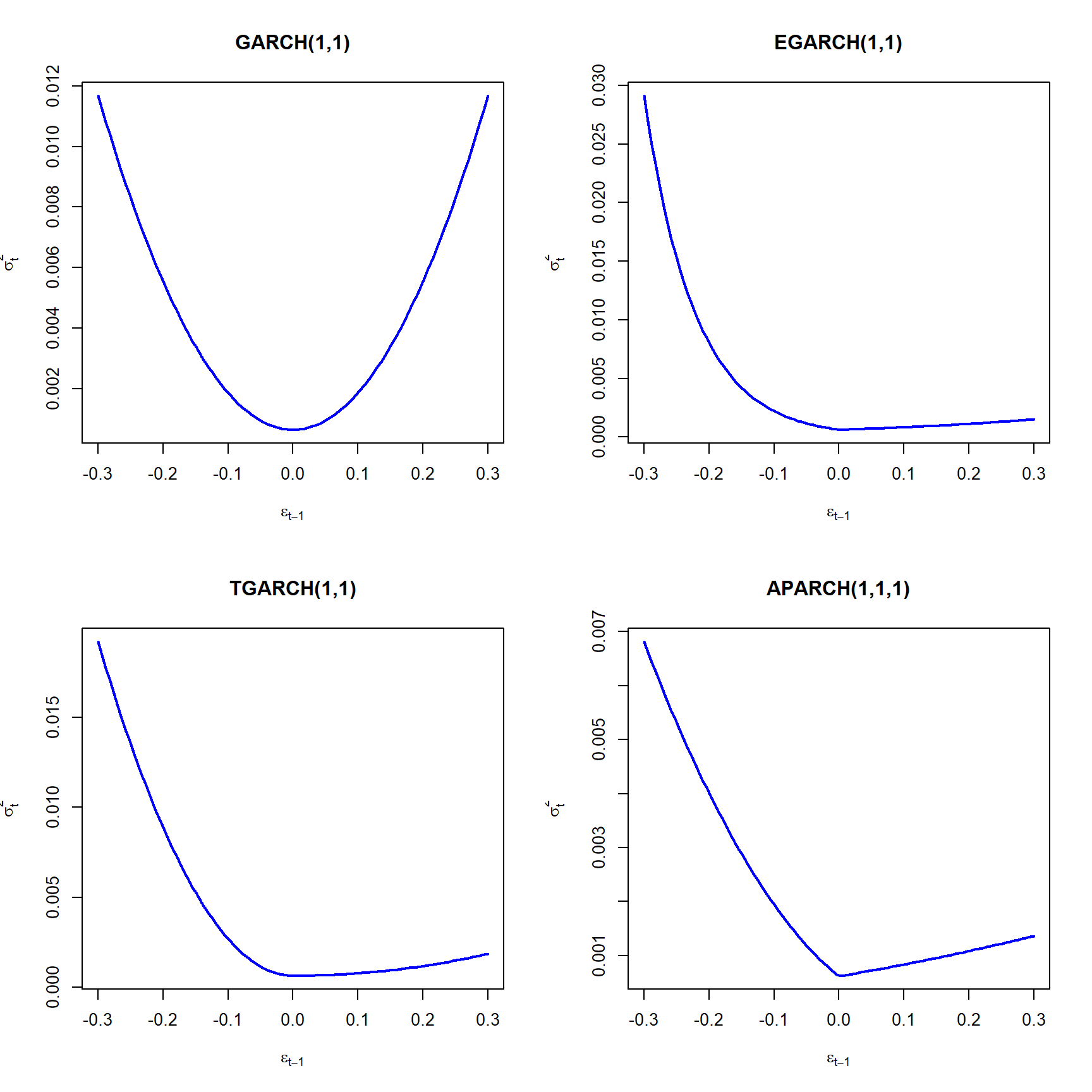

Modelo GARCH com erros não-normais

Vamos observar um modelo GARCH(1,1) normal, examinaremos os resíduos padronizados:

VALE.garch11.zt = residuals(VALE.garch11.fit)/sigma(VALE.garch11.fit)
VALE.garch11.zt = xts(VALE.garch11.zt, order.by=index(VALE.ret))
qqPlot(coredata(VALE.garch11.zt))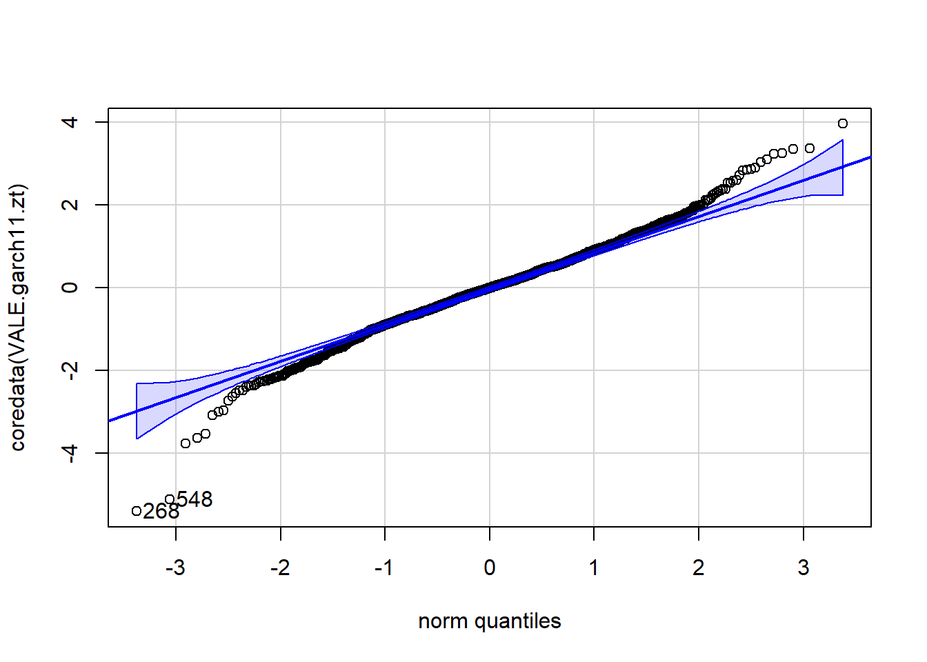

[1] 268 548

plot(VALE.garch11.fit, which=8)

plot(VALE.garch11.fit, which=9)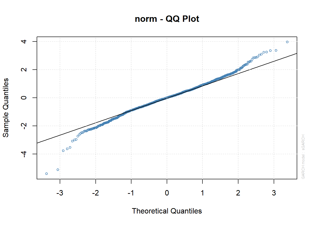

Rodaremos um modelo GARCH(1,1) com erros de Student \(t\):

garch11.t.spec = ugarchspec(variance.model = list(garchOrder=c(1,1)), 
                            mean.model = list(armaOrder=c(0,0)),
                            distribution.model = "std")
VALE.garch11.t.fit = ugarchfit(spec=garch11.t.spec, data=VALE.ret)                             
VALE.garch11.t.fit


*---------------------------------*
*          GARCH Model Fit        *
*---------------------------------*

Conditional Variance Dynamics   
-----------------------------------
GARCH Model : sGARCH(1,1)
Mean Model  : ARFIMA(0,0,0)
Distribution    : std 

Optimal Parameters
------------------------------------
        Estimate  Std. Error  t value Pr(>|t|)
mu      0.000510    0.000646  0.78967 0.429722
omega   0.000082    0.000032  2.52697 0.011505
alpha1  0.077329    0.023052  3.35461 0.000795
beta1   0.807590    0.060547 13.33824 0.000000
shape   6.563801    1.125766  5.83052 0.000000

Robust Standard Errors:
        Estimate  Std. Error  t value Pr(>|t|)
mu      0.000510    0.000633   0.8060 0.420244
omega   0.000082    0.000035   2.3304 0.019786
alpha1  0.077329    0.037766   2.0476 0.040604
beta1   0.807590    0.072977  11.0664 0.000000
shape   6.563801    1.222901   5.3674 0.000000

LogLikelihood : 3075 

Information Criteria
------------------------------------
                    
Akaike       -4.4887
Bayes        -4.4696
Shibata      -4.4887
Hannan-Quinn -4.4815

Weighted Ljung-Box Test on Standardized Residuals
------------------------------------
                        statistic p-value
Lag[1]                   0.003734  0.9513
Lag[2*(p+q)+(p+q)-1][2]  0.281145  0.8063
Lag[4*(p+q)+(p+q)-1][5]  1.695005  0.6920
d.o.f=0
H0 : No serial correlation

Weighted Ljung-Box Test on Standardized Squared Residuals
------------------------------------
                        statistic   p-value
Lag[1]                      15.55 8.029e-05
Lag[2*(p+q)+(p+q)-1][5]     15.95 2.460e-04
Lag[4*(p+q)+(p+q)-1][9]     17.14 1.066e-03
d.o.f=2

Weighted ARCH LM Tests
------------------------------------
            Statistic Shape Scale P-Value
ARCH Lag[3]    0.3973 0.500 2.000  0.5285
ARCH Lag[5]    0.6670 1.440 1.667  0.8335
ARCH Lag[7]    1.2800 2.315 1.543  0.8642

Nyblom stability test
------------------------------------
Joint Statistic:  0.8766
Individual Statistics:             
mu     0.1006
omega  0.2864
alpha1 0.2121
beta1  0.3080
shape  0.3454

Asymptotic Critical Values (10% 5% 1%)
Joint Statistic:         1.28 1.47 1.88
Individual Statistic:    0.35 0.47 0.75

Sign Bias Test
------------------------------------
                   t-value      prob sig
Sign Bias            1.453 1.465e-01    
Negative Sign Bias   4.634 3.922e-06 ***
Positive Sign Bias   0.199 8.423e-01    
Joint Effect        23.560 3.086e-05 ***


Adjusted Pearson Goodness-of-Fit Test:
------------------------------------
  group statistic p-value(g-1)
1    20     19.98       0.3956
2    30     25.29       0.6631
3    40     28.14       0.9014
4    50     39.02       0.8456


Elapsed time : 0.3038

plot(VALE.garch11.t.fit, which=9)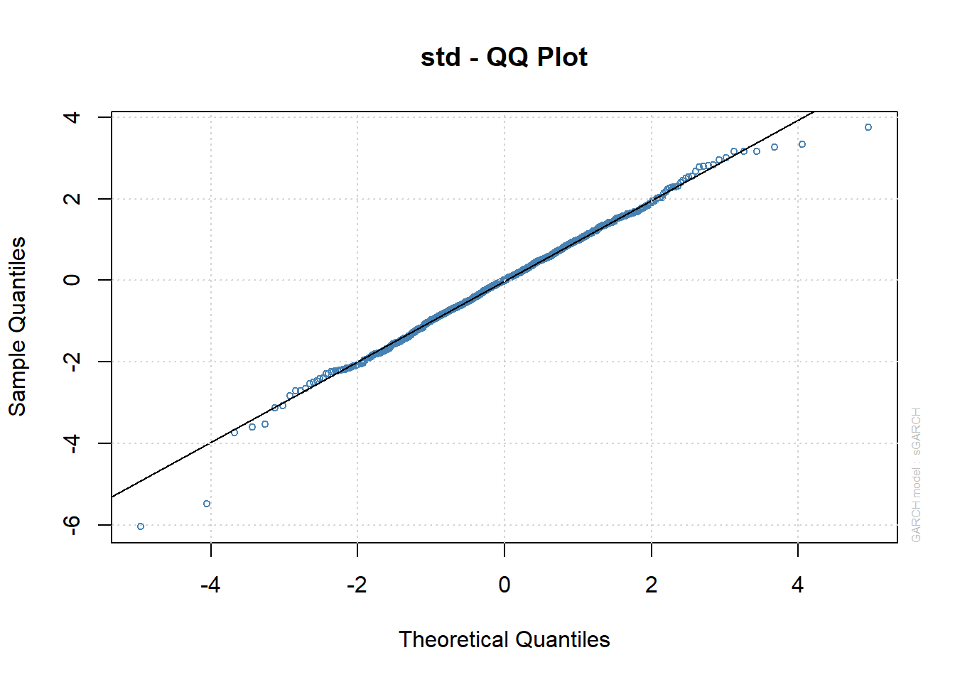

aparch11.1.t.spec = ugarchspec(variance.model = list(model="apARCH",
                                                     garchOrder=c(1,1)), 
                               mean.model = list(armaOrder=c(0,0)),
                               distribution.model = "std",
                               fixed.pars=list(delta=1))
VALE.aparch11.1.t.fit = ugarchfit(spec=aparch11.1.t.spec, data=VALE.ret)                             
VALE.aparch11.1.t.fit


*---------------------------------*
*          GARCH Model Fit        *
*---------------------------------*

Conditional Variance Dynamics   
-----------------------------------
GARCH Model : apARCH(1,1)
Mean Model  : ARFIMA(0,0,0)
Distribution    : std 

Optimal Parameters
------------------------------------
        Estimate  Std. Error  t value Pr(>|t|)
mu      0.000145    0.000647  0.22422 0.822584
omega   0.002495    0.000967  2.57914 0.009905
alpha1  0.082988    0.021633  3.83616 0.000125
beta1   0.842620    0.047924 17.58228 0.000000
gamma1  0.603759    0.192088  3.14313 0.001671
delta   1.000000          NA       NA       NA
shape   6.795048    1.197332  5.67516 0.000000

Robust Standard Errors:
        Estimate  Std. Error  t value Pr(>|t|)
mu      0.000145    0.000655  0.22145 0.824740
omega   0.002495    0.001224  2.03781 0.041569
alpha1  0.082988    0.025608  3.24064 0.001193
beta1   0.842620    0.060979 13.81829 0.000000
gamma1  0.603759    0.180442  3.34600 0.000820
delta   1.000000          NA       NA       NA
shape   6.795048    1.198521  5.66953 0.000000

LogLikelihood : 3081 

Information Criteria
------------------------------------
                    
Akaike       -4.4961
Bayes        -4.4732
Shibata      -4.4961
Hannan-Quinn -4.4875

Weighted Ljung-Box Test on Standardized Residuals
------------------------------------
                        statistic p-value
Lag[1]                   0.003469  0.9530
Lag[2*(p+q)+(p+q)-1][2]  0.340440  0.7736
Lag[4*(p+q)+(p+q)-1][5]  1.592027  0.7173
d.o.f=0
H0 : No serial correlation

Weighted Ljung-Box Test on Standardized Squared Residuals
------------------------------------
                        statistic   p-value
Lag[1]                      18.62 1.591e-05
Lag[2*(p+q)+(p+q)-1][5]     19.00 3.644e-05
Lag[4*(p+q)+(p+q)-1][9]     20.07 1.924e-04
d.o.f=2

Weighted ARCH LM Tests
------------------------------------
            Statistic Shape Scale P-Value
ARCH Lag[3]    0.1486 0.500 2.000  0.6999
ARCH Lag[5]    0.3035 1.440 1.667  0.9393
ARCH Lag[7]    0.9906 2.315 1.543  0.9151

Nyblom stability test
------------------------------------
Joint Statistic:  0.8841
Individual Statistics:              
mu     0.07869
omega  0.16672
alpha1 0.17589
beta1  0.16925
gamma1 0.11133
shape  0.30942

Asymptotic Critical Values (10% 5% 1%)
Joint Statistic:         1.49 1.68 2.12
Individual Statistic:    0.35 0.47 0.75

Sign Bias Test
------------------------------------
                   t-value      prob sig
Sign Bias           1.7339 8.317e-02   *
Negative Sign Bias  4.1472 3.574e-05 ***
Positive Sign Bias  0.1362 8.917e-01    
Joint Effect       17.3662 5.942e-04 ***


Adjusted Pearson Goodness-of-Fit Test:
------------------------------------
  group statistic p-value(g-1)
1    20     15.95       0.6608
2    30     29.41       0.4438
3    40     24.05       0.9711
4    50     38.14       0.8690


Elapsed time : 1.231

plot(residuals(VALE.aparch11.1.t.fit))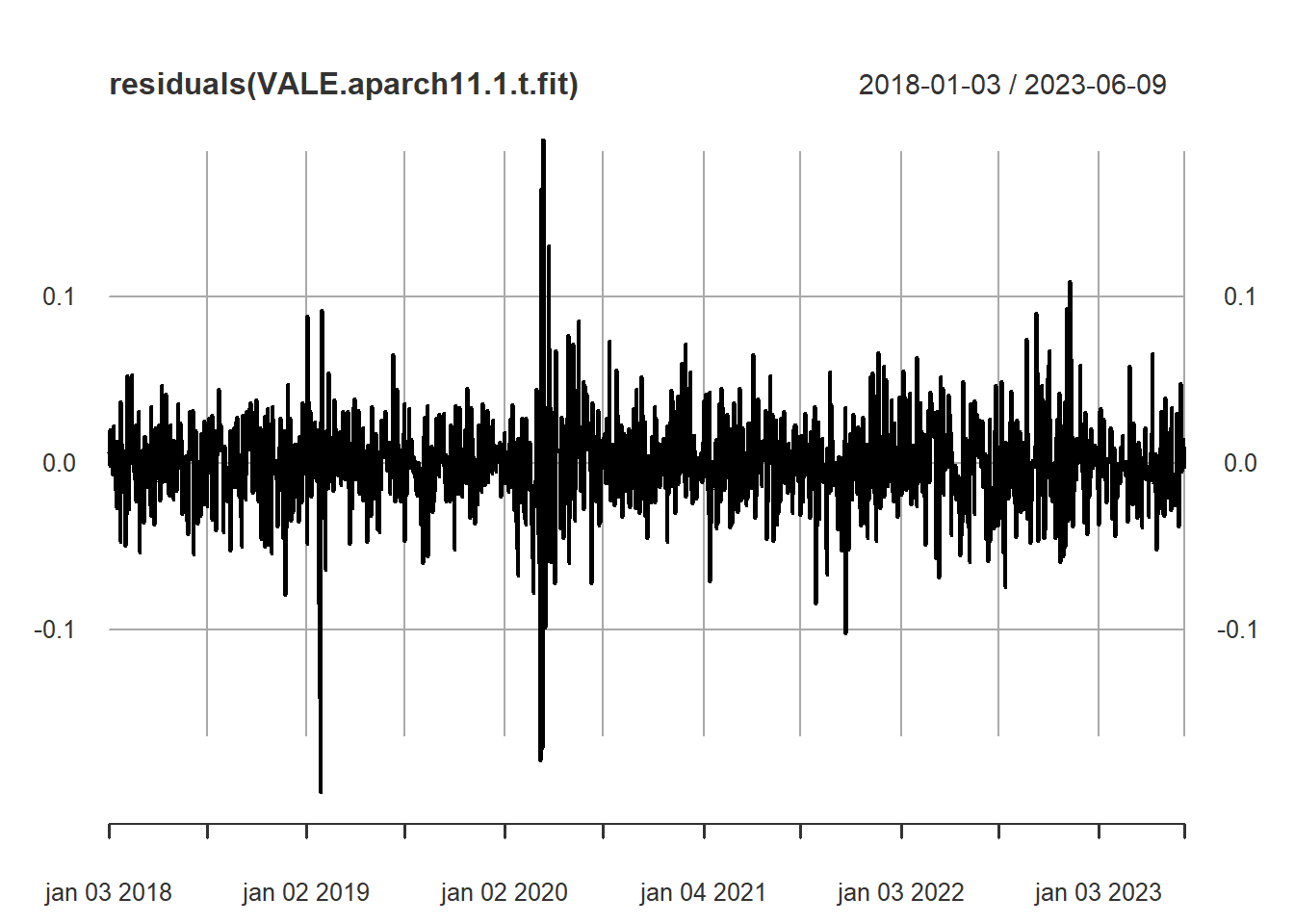

Ajustamos uma \(t\) enviesada:

garch11.st.spec = ugarchspec(variance.model = list(garchOrder=c(1,1)), 
                            mean.model = list(armaOrder=c(0,0)),
                            distribution.model = "sstd")
VALE.garch11.st.fit = ugarchfit(spec=garch11.st.spec, data=VALE.ret)                             
VALE.garch11.st.fit


*---------------------------------*
*          GARCH Model Fit        *
*---------------------------------*

Conditional Variance Dynamics   
-----------------------------------
GARCH Model : sGARCH(1,1)
Mean Model  : ARFIMA(0,0,0)
Distribution    : sstd 

Optimal Parameters
------------------------------------
        Estimate  Std. Error  t value Pr(>|t|)
mu      0.000340    0.000683  0.49827 0.618294
omega   0.000080    0.000032  2.51984 0.011741
alpha1  0.076986    0.022903  3.36144 0.000775
beta1   0.809743    0.059818 13.53670 0.000000
skew    0.971957    0.036344 26.74360 0.000000
shape   6.592137    1.135063  5.80773 0.000000

Robust Standard Errors:
        Estimate  Std. Error  t value Pr(>|t|)
mu      0.000340    0.000673   0.5054 0.613279
omega   0.000080    0.000034   2.3344 0.019573
alpha1  0.076986    0.037494   2.0533 0.040042
beta1   0.809743    0.072072  11.2351 0.000000
skew    0.971957    0.037452  25.9523 0.000000
shape   6.592137    1.221276   5.3977 0.000000

LogLikelihood : 3076 

Information Criteria
------------------------------------
                    
Akaike       -4.4876
Bayes        -4.4647
Shibata      -4.4877
Hannan-Quinn -4.4790

Weighted Ljung-Box Test on Standardized Residuals
------------------------------------
                        statistic p-value
Lag[1]                   0.003709  0.9514
Lag[2*(p+q)+(p+q)-1][2]  0.279837  0.8070
Lag[4*(p+q)+(p+q)-1][5]  1.692357  0.6926
d.o.f=0
H0 : No serial correlation

Weighted Ljung-Box Test on Standardized Squared Residuals
------------------------------------
                        statistic   p-value
Lag[1]                      15.44 8.529e-05
Lag[2*(p+q)+(p+q)-1][5]     15.84 2.634e-04
Lag[4*(p+q)+(p+q)-1][9]     17.04 1.132e-03
d.o.f=2

Weighted ARCH LM Tests
------------------------------------
            Statistic Shape Scale P-Value
ARCH Lag[3]    0.3944 0.500 2.000   0.530
ARCH Lag[5]    0.6753 1.440 1.667   0.831
ARCH Lag[7]    1.2759 2.315 1.543   0.865

Nyblom stability test
------------------------------------
Joint Statistic:  1.289
Individual Statistics:             
mu     0.0969
omega  0.2857
alpha1 0.2098
beta1  0.3087
skew   0.5322
shape  0.3299

Asymptotic Critical Values (10% 5% 1%)
Joint Statistic:         1.49 1.68 2.12
Individual Statistic:    0.35 0.47 0.75

Sign Bias Test
------------------------------------
                   t-value      prob sig
Sign Bias           1.4998 1.339e-01    
Negative Sign Bias  4.6772 3.197e-06 ***
Positive Sign Bias  0.2336 8.153e-01    
Joint Effect       23.9089 2.610e-05 ***


Adjusted Pearson Goodness-of-Fit Test:
------------------------------------
  group statistic p-value(g-1)
1    20     15.95       0.6608
2    30     25.42       0.6562
3    40     28.32       0.8970
4    50     36.02       0.9162


Elapsed time : 0.4376

plot(VALE.garch11.st.fit, which=9)

Plotamos os gráficos dos modelos da família ARCH

VALE.garch11.fcst = ugarchforecast(VALE.garch11.fit, n.ahead=250)
VALE.garch11.t.fcst = ugarchforecast(VALE.garch11.t.fit, n.ahead=250)
VALE.aparch11.1.fcst = ugarchforecast(VALE.aparch11.1.fit, n.ahead=250)
VALE.aparch11.1.t.fcst = ugarchforecast(VALE.aparch11.1.t.fit, n.ahead=250)

Ploto os gráficos

par(mfrow=c(2,2))

plot(sigma(VALE.garch11.fcst), type="l", col="blue")

plot(sigma(VALE.garch11.t.fcst), type="l", col="blue")

plot(sigma(VALE.aparch11.1.fcst), type="l", col="blue")

plot(sigma(VALE.aparch11.1.t.fcst), type="l", col="blue")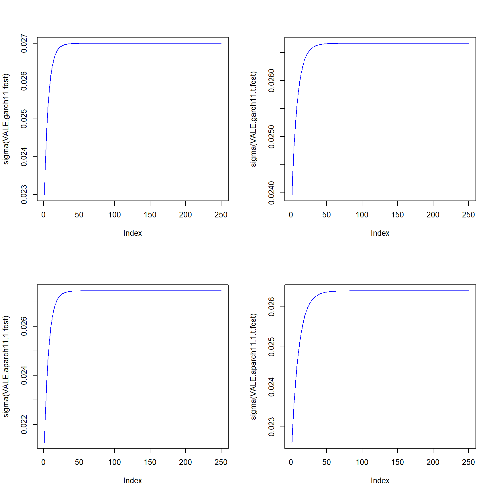

Extraio as projeções de volatilidades:

#VALE.garch11.sigma = as.data.frame(VALE.garch11.fcst)$sigma
#VALE.garch11.t.sigma = as.data.frame(VALE.garch11.t.fcst)$sigma
#VALE.aparch11.1.sigma = as.data.frame(VALE.aparch11.1.fcst)$sigma
#VALE.aparch11.1.t.sigma = as.data.frame(VALE.aparch11.1.t.fcst)$sigma

#ymax = max(VALE.garch11.sigma,VALE.garch11.t.sigma,VALE.aparch11.1.sigma, VALE.aparch11.1.t.sigma)
#ymin = min(VALE.garch11.sigma,VALE.garch11.t.sigma,VALE.aparch11.1.sigma, VALE.aparch11.1.t.sigma)

#plot.ts(VALE.garch11.sigma, main="Projeções de Volatilidades",
 #       ylim=c(ymin,ymax), col="black", 
  #      lwd=2, ylab="sigma(t+h|t)", xlab="h")
#lines(VALE.garch11.t.sigma, col="blue", lwd=2)
#lines(VALE.aparch11.1.sigma, col="green", lwd=2)
#lines(VALE.aparch11.1.t.sigma, col="red", lwd=2)
#legend(x="topleft", legend=c("GARCH-n", "GARCH-t", "APARCH-n", "APARCH-t"),
 #      col=c("black", "blue","green","red"), lwd=2, lty = "solid")

Reajusta os modelos, deixando 100 observações fora da amostra para estatísticas de avaliação de previsão

VALE.garch11.fit = ugarchfit(spec=garch11.spec, data=VALE.ret,
                             out.sample=100)
VALE.garch11.t.fit = ugarchfit(spec=garch11.t.spec, data=VALE.ret,
                               out.sample=100)
VALE.aparch11.1.fit = ugarchfit(aparch11.1.spec, VALE.ret,
                                out.sample=100)
VALE.aparch11.1.t.fit = ugarchfit(spec=aparch11.1.t.spec, data=VALE.ret,
                                  out.sample=100)

Compara a persistência com a variância incondicional:

c.mat = matrix(0, 4, 2)
colnames(c.mat) = c("Persistence", "E[sig(t)]")
rownames(c.mat) = c("GARCH-n", "GARCH-t", "APARCH-n","APARCH-t")
c.mat["GARCH-n","Persistence"] = persistence(VALE.garch11.fit)
c.mat["GARCH-t","Persistence"] = persistence(VALE.garch11.t.fit)
c.mat["APARCH-n","Persistence"] = persistence(VALE.aparch11.1.fit)
c.mat["APARCH-t","Persistence"] = persistence(VALE.aparch11.1.t.fit)

c.mat["GARCH-n","E[sig(t)]"] = sqrt(uncvariance(VALE.garch11.fit))
c.mat["GARCH-t","E[sig(t)]"] = sqrt(uncvariance(VALE.garch11.t.fit))
c.mat["APARCH-n","E[sig(t)]"] = sqrt(uncvariance(VALE.aparch11.1.fit))
c.mat["APARCH-t","E[sig(t)]"] = sqrt(uncvariance(VALE.aparch11.1.t.fit))

c.mat

         Persistence E[sig(t)]
GARCH-n       0.8402   0.02746
GARCH-t       0.8746   0.02709
APARCH-n      0.8522   0.02784
APARCH-t      0.8992   0.02672

Finaliza computando 100 previsões dinâmicas 1 passo à frente:

VALE.garch11.fcst = ugarchforecast(VALE.garch11.fit, n.roll=100, n.ahead=1)
VALE.garch11.t.fcst = ugarchforecast(VALE.garch11.t.fit, n.roll=100, n.ahead=1)
VALE.aparch11.1.fcst = ugarchforecast(VALE.aparch11.1.fit, n.roll=100, n.ahead=1)
VALE.aparch11.1.t.fcst = ugarchforecast(VALE.aparch11.1.t.fit, n.roll=100, n.ahead=1)

Vamos ver os resultados para os retornos esperados pelos 4 modelos ajustados:

VALE.garch11.fcst


*------------------------------------*
*       GARCH Model Forecast         *
*------------------------------------*
Model: sGARCH
Horizon: 1
Roll Steps: 100
Out of Sample: 1

0-roll forecast [T0=2023-01-17]:
       Series   Sigma
T+1 0.0008252 0.02441

VALE.garch11.t.fcst


*------------------------------------*
*       GARCH Model Forecast         *
*------------------------------------*
Model: sGARCH
Horizon: 1
Roll Steps: 100
Out of Sample: 1

0-roll forecast [T0=2023-01-17]:
       Series   Sigma
T+1 0.0008341 0.02453

VALE.aparch11.1.fcst


*------------------------------------*
*       GARCH Model Forecast         *
*------------------------------------*
Model: apARCH
Horizon: 1
Roll Steps: 100
Out of Sample: 1

0-roll forecast [T0=2023-01-17]:
      Series   Sigma
T+1 2.16e-05 0.02453

VALE.aparch11.1.t.fcst


*------------------------------------*
*       GARCH Model Forecast         *
*------------------------------------*
Model: apARCH
Horizon: 1
Roll Steps: 100
Out of Sample: 1

0-roll forecast [T0=2023-01-17]:
       Series   Sigma
T+1 0.0004423 0.02365

Com os dados observados, comparamos o de melhor ajuste:

# Obtem comparativo de previsao estatistica
fcst.list = list(garch11=VALE.garch11.fcst,
                 garch11.t=VALE.garch11.t.fcst,
                 aparch11.1=VALE.aparch11.1.fcst,
                 aparch11.t.1=VALE.aparch11.1.t.fcst)
fpm.mat = sapply(fcst.list, fpm)
fpm.mat

    garch11   garch11.t aparch11.1 aparch11.t.1
MSE 0.0004522 0.0004523 0.0004476  0.0004498   
MAE 0.01625   0.01625   0.01612    0.01618     
DAC 0.43      0.43      0.43       0.43

Referências

Graves, Spencer. 2014. FinTS: Companion to Tsay (2005) Analysis of Financial Time Series. https://CRAN.R-project.org/package=FinTS.

Ghalanos, Alexios. 2015. Rugarch: Univariate Garch Models. https://CRAN.R-project.org/package=rugarch.

Análise econométrica em tempo real: Modelos família ARCH para dados financeiros

Rodrigo H. Ozon

21/09/2020

Resumo

Introdução

`PBR` Preço de Fechamento do pregão

`PBR` Volume negociado

`^BVSP` Preço de Fechamento do pregão

`^BVSP` Volume negociado

`VALE` Preço de Fechamento do pregão

`VALE` Volume negociado

Volatilidade Variável no Tempo e Modelos ARCH

O modelo ARCH

Rodando o modelo ARCH e GARCH para os dados da VALE

O modelo GARCH

Outro script para a News Impact Curve

GARCH Assimétrico

Modelo EGARCH de Nelson

Modelo GJR GARCH

Modelo APARCH

Comparando as News Impact Curves

Modelo GARCH com erros não-normais

Plotamos os gráficos dos modelos da família ARCH

Referências

Análise econométrica em tempo real: Modelos família ARCH para dados financeiros

Rodrigo H. Ozon

21/09/2020

Resumo

Introdução

PBR Preço de Fechamento do pregão

PBR Volume negociado

^BVSP Preço de Fechamento do pregão

^BVSP Volume negociado

VALE Preço de Fechamento do pregão

VALE Volume negociado

Volatilidade Variável no Tempo e Modelos ARCH

O modelo ARCH

Rodando o modelo ARCH e GARCH para os dados da VALE

O modelo GARCH

Outro script para a News Impact Curve

GARCH Assimétrico

Modelo EGARCH de Nelson

Modelo GJR GARCH

Modelo APARCH

Comparando as News Impact Curves

Modelo GARCH com erros não-normais

Plotamos os gráficos dos modelos da família ARCH

Referências

`PBR` Preço de Fechamento do pregão

`PBR` Volume negociado

`^BVSP` Preço de Fechamento do pregão

`^BVSP` Volume negociado

`VALE` Preço de Fechamento do pregão

`VALE` Volume negociado